Lattice Model Editor: Heisenberg Ladder

In Aleph quantum many body systems can be represented by the model class, which stores a geometry and interactions on that geometry, along with the observables to be computed. Many of the most interesting quantum systems are lattice models in one or two dimensions. The Lattice Model Editor is a graphical tool for defining a lattice model in one or two dimensions. This tutorial explains how to use the lattice model editor to build a Heisenberg Ladder and compute its magnetization.

Defining the Lattice

When opening the lattice editor, we're presented with a canvas containing a dashed box. This dashed box represents a unit cell in the lattice (see here for a review of lattices in Aleph),

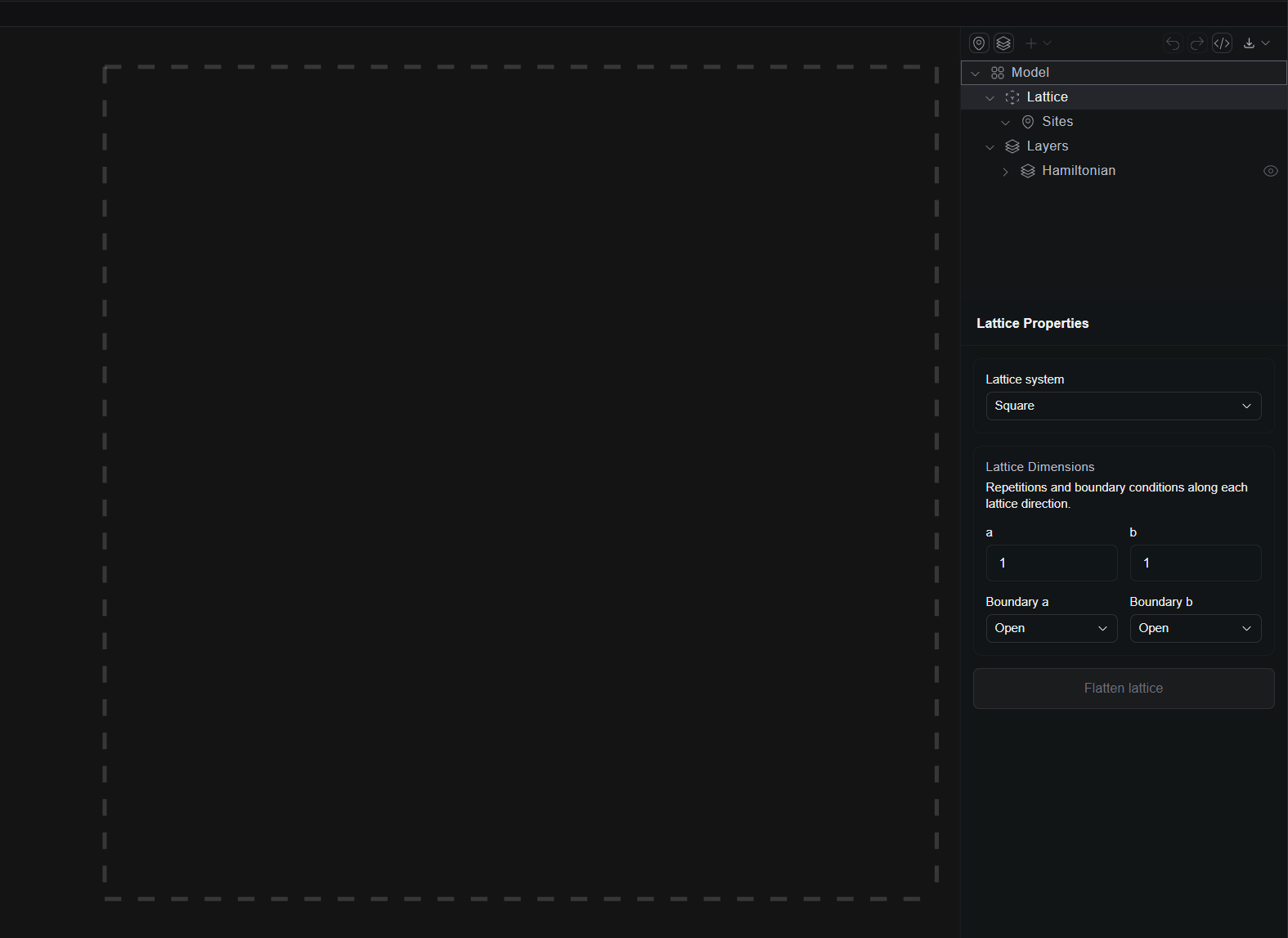
Defining the Lattice

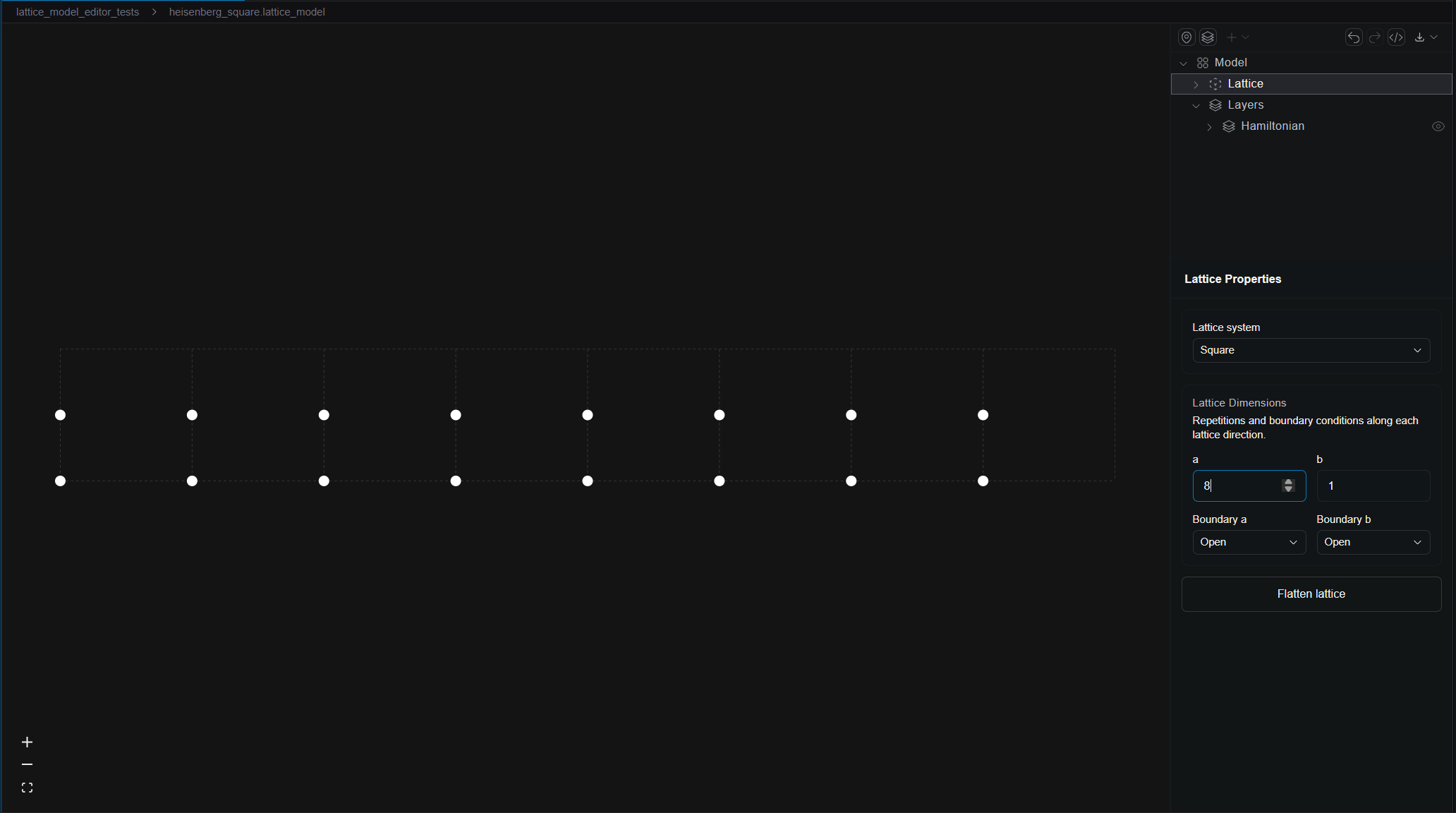
Selecting Lattice on the right hand side panel brings up the lattice proerty sheet. Here we can change the dimensions of the lattice by varying $a$ and $b$, as well as the primitive vectors by selecting from one of the five two dimensional Bravais lattice systems. For now we'll leave these untouched and come back later to resize the lattice.

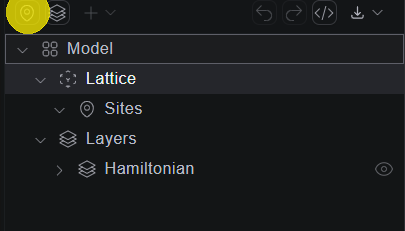
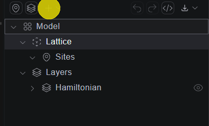
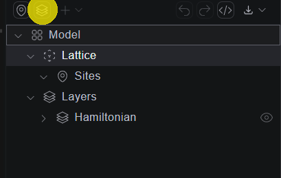
The first step to building a lattice is to add some atomic basis sites. This can be done with the Add Site button on the right side panel highlights in yellow below,

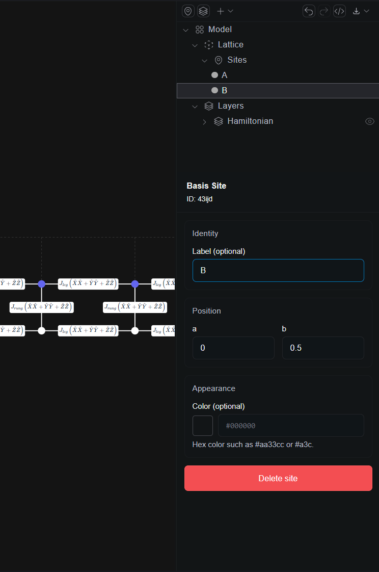
The sites then appear on the unit cell. Since we're making a ladder, let's represent the ladder as a two site basis.

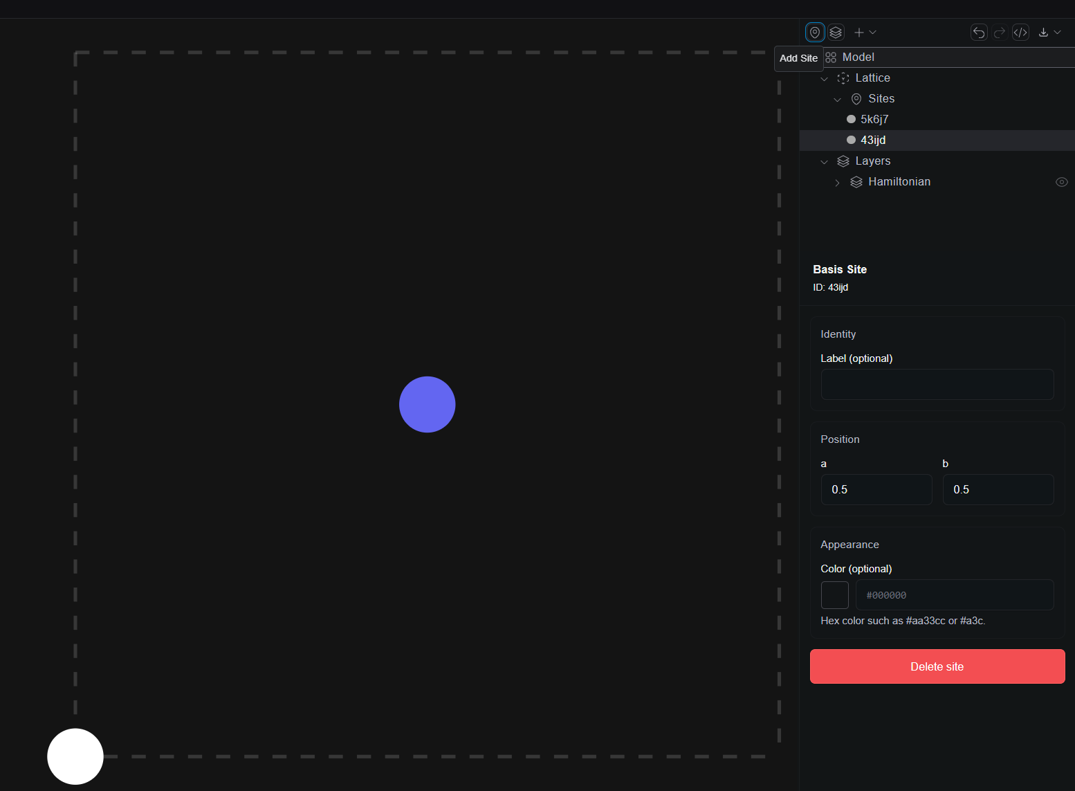
Notice that on the right hand panel under the lattice heading the sites now appear with randomly assigned labels. These labels can be modified for convenience later.

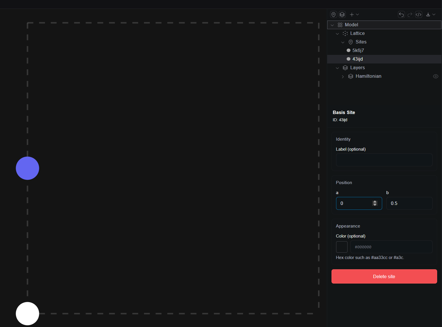
There are two ways to position the basis sites, first by clicking and dragging, and second by adjusting the $a$ and $b$ positions on the Basis Site property sheet, displayed on the lower right hand side,

Now that we have our unit cell, we can extend the ladder along the $a$ direction by selecting Lattice on the right hand side panel and setting the value of $a$ under dimensions,

Adding Interactions

To add interactions to the model, we can hold shift and select the one or more sites that will participate in the interaction and clicking the Add Interaction button highlighted below,

When we click Add Interaction we can choose between adding a new interaction or adding an interaction from an existing interaction. Since there are no existing interactions, we'll add a new interaction.

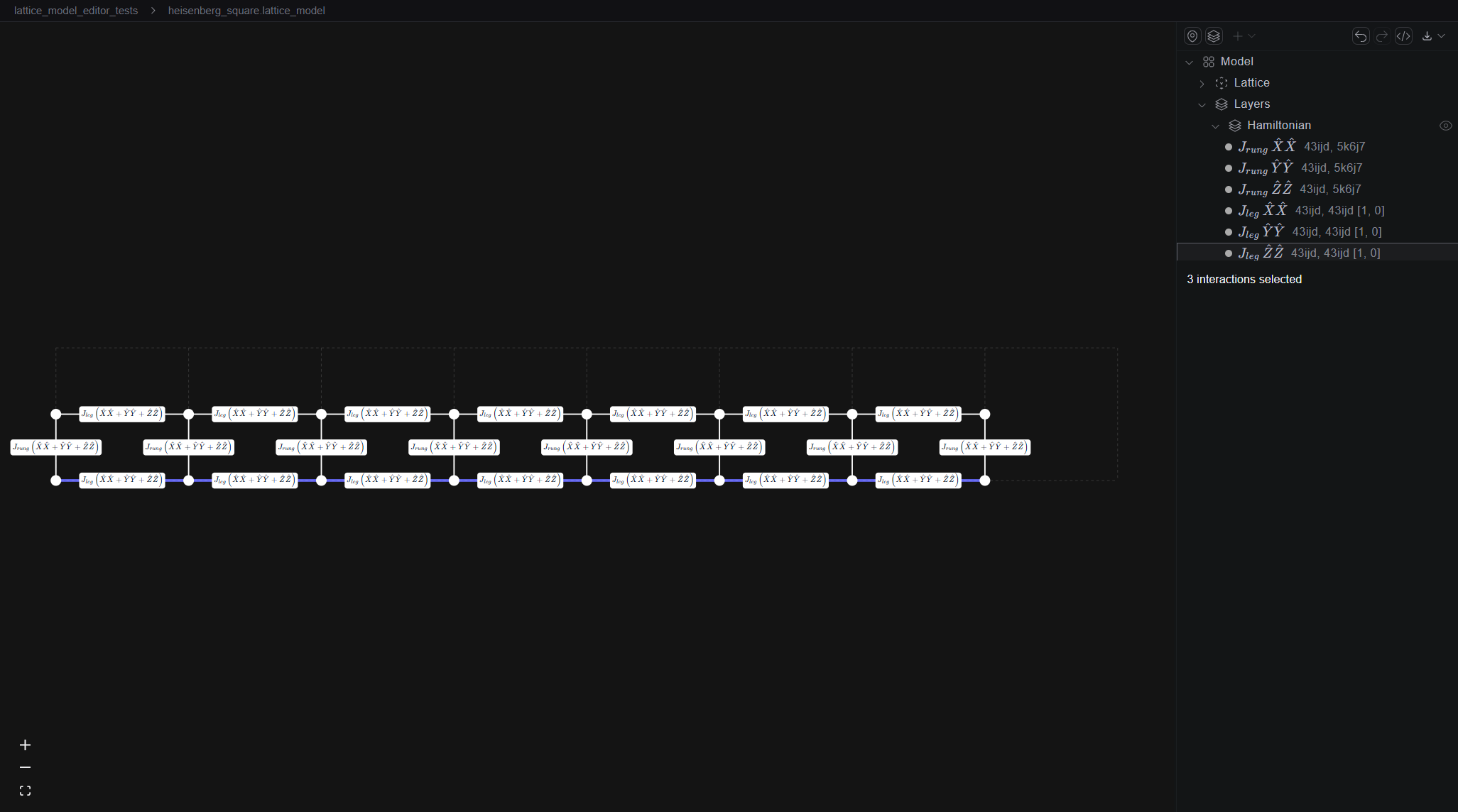
Because the model is assumed to have the symmetry of the lattice, we only need to define a single representative interaction, and the editor will interpret it as being repeated on all sites equivalent under lattice translations. Let's demonstrate this by adding the rung interaction,

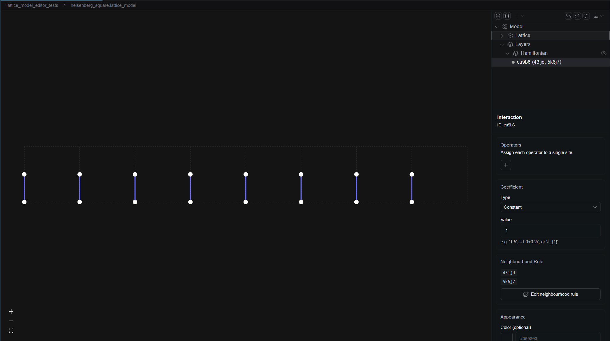
Focusing on the right panel, we can see that the interaction, along with the sites participating in the interaction has appeared in the right hand side tree under the Hamiltonian layer. This layer is the default place for interactions to be defined. Below, we can also see the property sheet for the interaction.

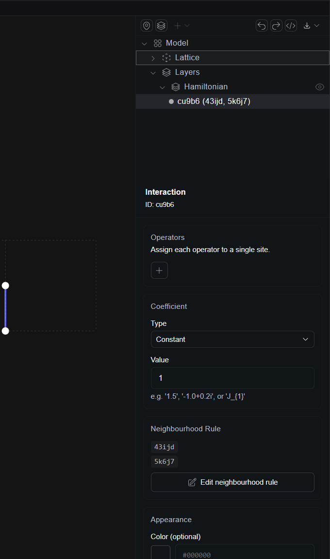
This is the place where we can define the operators that act on the sites, as well as the coefficient associated with the interaction. Clicking the plus button on the Operators header allows us to add a single site operator, and to select which site that operator acts on, as shown below,

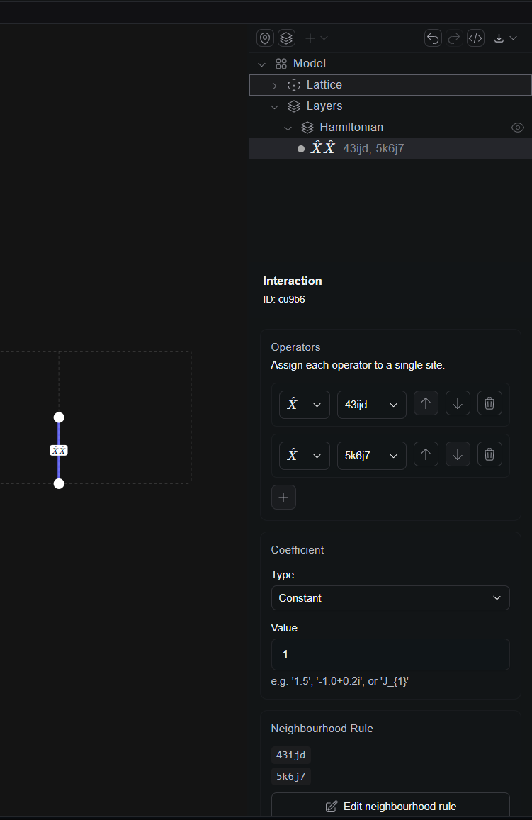
In the above screenshot, we can also see the Neighbourhood Rule header, which is associated to the neighbourhood rules that can be added to a model. Unlike in Aleph script where neighbourhood rules are defined by the displacements from the reference site, in the editor, the neighbourhood rule is defined by the sites it acts on, with the first site corresponding to the reference site. The two representations are dual to one another.

By default the coefficient attached to this interaction is $1.0$. It's possible to set the coefficient to any complex value, in which case it's the equivalent of calling,

my_model.add(interaction(constant, [X, X], "neighbourhood"))

but often we want to group interactions under a common coefficient. To achieve this we can select Label under the coefficient Type menu, and set the value to a label that will render as TeX in the editor, as shown below.

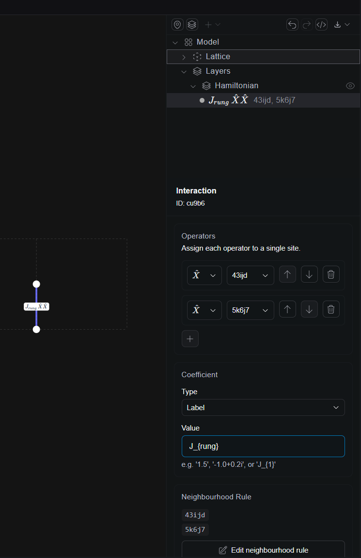
When it comes time to load our model into Aleph, the label J_{rung} will be declared as an unregistered label, we can then set the label to any valid coefficient (either a complex number or coefficient) via,

my_model.set_coefficient("J_{rung}", J_rung_value)

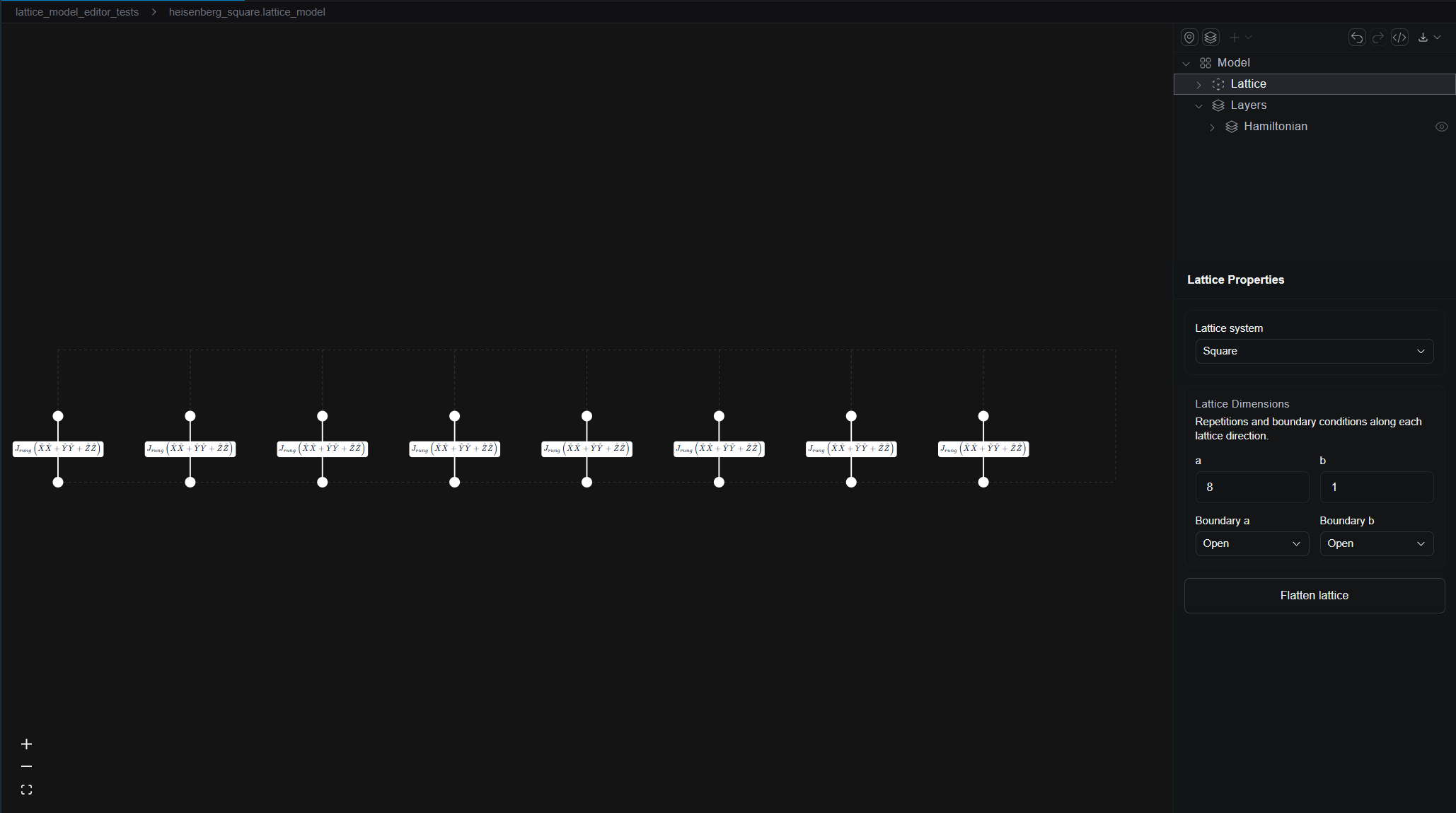
We can repeat the process described above, selecting the two representative sites and selecting Add Interaction. Since we've already defined a rung interaction, we can save some time by selecing add interaction from existing... and selecting the interaction we just defined. To define a Heisenberg coupling, we need $Y$ and $Z$ exchange interactions. Notice that when we add interactions with the same coefficient, the label on the canvas naturally groups them together.

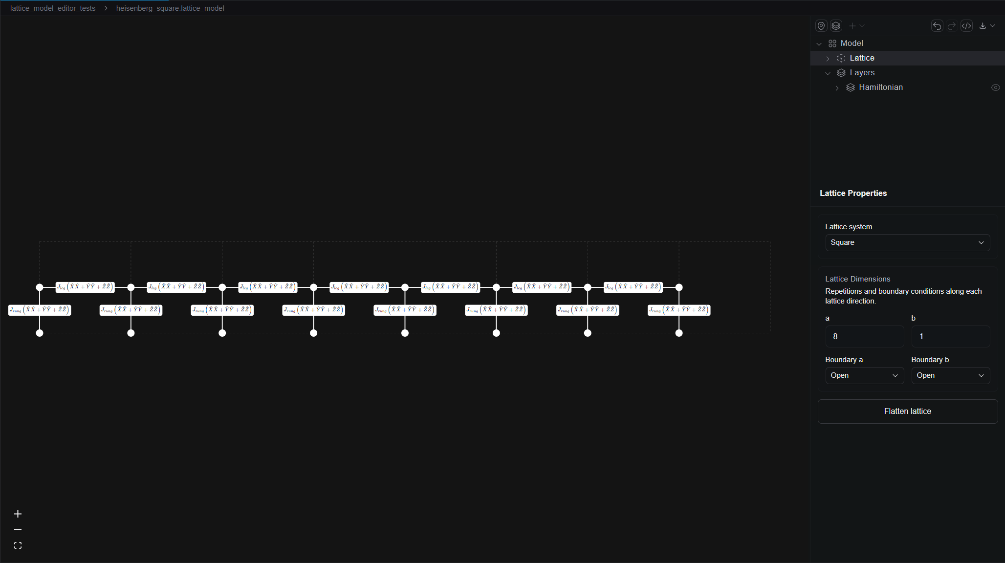
We can easily add the two leg interactions by selecting two candidate sites from each unit cell and clicking Add Interaction, once again we add interaction from existing..., this time selecting all three of the exchange coupling for the rung. We can now change the label from J_{rung} to J_{leg}, allowing us to tune the relative coupling in our subsequent analysis. Finally, we can complete our Heisenberg ladder by adding the last leg interaction,

Before we move on, let's clean up our interface by giving the labels $A$ and $B$ to the two sites in the basis. By clicking on the sites under on the tree on the right hand site, we can bring up the property sheet for the basis sites and add labels as shown below,

Adding Observables

Now that we've defined the interactions in the Hamiltonian, we can add some observables to the model. First we can add an observable layer, using the highlighted button below,

Let's define an observable for the total magnetization along the $z$ axis. The magnetization is a sum over single site interactions. To add these interactions we can select each site and click the Add Interaction button, just as we did for the Hamiltonian. In this case we can leave the constant factor in from of the operator as $1.0$. If the interaction was mistakenly added under the Hamiltonian, we can click and drag the operator under the correct observable,

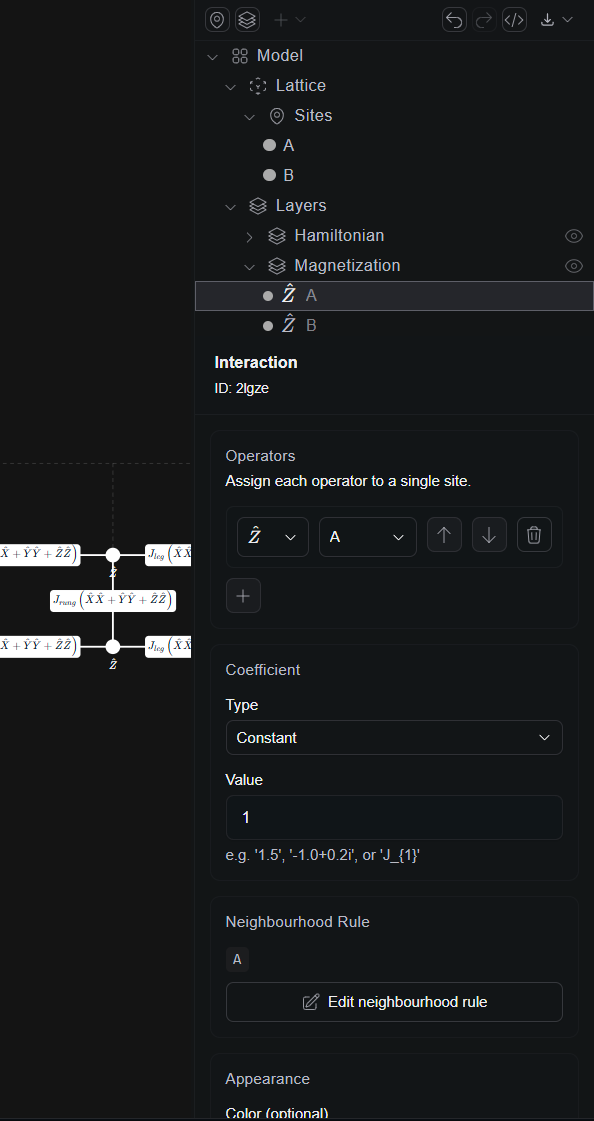
This is equivalent to calling

my_model.add_observable("Magnetization", interaction(1.0, Z, "A"))
my_model.add_observable("Magnetization", interaction(1.0, Z, "B"))

By now the canvas has become quite busy. One the right panel next to the name of each layer is a button that can hide those layers, allowing users to focus on particular observables.

The model file can now be loaded into Aleph script. If we save our lattice_model file as heisenberg_ladder.lattice_model, then we can open a script heisenberg_ladder.aleph with the line

var my_model = model("heisenberg_ladder.lattice_model");

You can also drag and drop the .lattice_model file directly from the left hand side panel to the line on the .aleph file where you want to load the model. Before we can use this model, we have to register the coefficients. To see which coefficient labels still need definition, we can write,

print(my_model.unresolved_labels()) //-> [J_{leg}, J_{rung}]

We can now set these labels to any valid coefficient value using, for example,

my_model.set_coefficient("J_{leg}", 1.0+0.0i)
my_model.set_coefficient("J_{rung}", 1.0+0.0i)

For more details on how to use the model, refer to the dedicated model concept page

Documentation Contributors

James Lambert