The SSH Model And The Adiabatic Charge Pump

The Su-Schrieffer-Heeger (SSH) Model And Edge Modes

Topological physics is at the heart of many exotic phenomena in condensed matter system. Differing from their strongly interacting counterparts, these non-interacting systems provide a platform for the bulk and edge properties of a material to be determined by some topological invariant. One of the first models that explored this was the one dimensional SSH model with open boundary conditions

$$v \sum_{i=1}^N (c^\dag_{i,A} c_{i,B} + \mathrm{h.c.}) + w\sum_{i=1}^{N-1} (c^{\dag}_{i+1,A}c_{i,B} + \mathrm{h.c.}).$$

This is a toy model that describes a single electron in polyacetylene, a linear molecule of carbon atoms with two inequivalent kinds of bonds. The unit cell for this model is comprised of two different sublattice sites that we label as $A$ and $B$. An equivalent way to view this is to consider each unit cell as one site, with two orbitals or modes in the unit cell. As such for a chain of $N$ unit cells, there will be a total $2N$ total modes where the electron can be.

note

When expressing free fermionic systems as a hamiltonian, they must be cast as real-space hopping models. Expressions containing pauli matrices defining the interactions for the internal site degrees of freedom are not currently supported, they must also be cast in real-space.

The first term in the hamiltonian is the intracell hopping between the two modes in the cells with amplitude $v$ while the second term is intercell hopping between unit cells with amplitude $w$. It should be noted that the hopping between cells only connects different modes to each other, that is there are no $c^{\dag}_{i+1,A}c_{i,A}$ or $c^{\dag}_{i+1,B}c_{i,B}$ terms. The system has two gapped phases: the trivial phase $|v| > |w|$, the topological one for $|v| < |w|$, and the gap closes when $|v| = |w|$.

In the trivial phase the electron hopping in the unit cell dominates (the so called dimerized limit) while in the topological phase the hopping between unit cells does. In open boundary conditions there exists edge modes, eigenstates of the hamiltonian with near zero energy that are exponentially localized to one edge of the chain. These are protected by topology in the sense that one can define a winding number, the number of times the real space 3D vector

$$\bold{d}(k) = (v+wcos(k),wsin(k),0)$$

encircles the origin as $k$ is moved through the brillouin zone. This can be seen by looking at the model in momentum space, where it takes the form $H(k) = \bold{d}(k) \cdot \bold{\sigma}$ where $\bold{\sigma} = (\sigma_x,\sigma_y,\sigma_z)$. In the trivial phase the vector does not contain the origin, while in the topological phase it does. As long as $|v| < |w|$, the origin is always encircled and thus the open boundary condition zero edge modes are protected.

A Protocol To Move The Edge States

One can promote the static parameters of the SSH model to vary with time

$$v(t) \sum_{i=1}^N (c^\dag_{i,A} c_{i,B} + h.c) + w(t)\sum_i^{N-1} (c^{\dag}_{i+1,A}c_{i,B} + h.c) + u(t) \sum_i^N (n_{i,A} - n_{i,B})$$

with $v(t) = 1 +\cos(\omega t)$ , $w(t) = 1$ , $u(t) = \sin(\omega t)$. This version of the SSH chain is called the Rice-Mele model and is similar to the static model, except for the onsite potential and the time dependence. With this particular scheme, when the model undergoes one cycle the edge modes get swapped, pumping one mode from one of the two energy "bands" to the other.

Getting the instantaneous Spectrum

We can see this numerically by obtaining the spectrum of this model as a function of time. We first start by constructing our single particle hamiltonian by making an operator sum corresponding to our expression:

def make_sum(integer num_sites, real t, real pump_frequency)
{
    var H = operator_sum(as_real)
    var vt = 1 + cos(pump_frequency*t)
    var ut = sin(pump_frequency*t)
    var wt = 1
    for (var i = 0; i < num_sites; ++i)
    {
        var A = 2 * i       // mode a site
        var B = 2 * i + 1   // mode b site

        H +=  vt * Hop(A, B)

        if (i < (num_sites - 1))
        {
            H += wt * Hop(B, B + 1)
        }

        H += ut * Number(A)
        H += -ut * Number(B)
    }

    return H
}

In this function we automate the construction of our operator expression by passing it the number of total sites we have in the system, the value of the time parameter and the frequency of the cycle. Note that we treat $A$ and $B$ modes as separate sites, even sites are all $A$ modes while odd sites are $B$ modes.

tip

You can extend this ordering scheme for 1D systems to add more modes by making blocks of your unit cell and indexing using the modulus operator. For 2D systems, the lattice class can help by using the basis system allowing you to make unit cells and specifying the position of the basis.

Next we set our parameters for the simulation, feel free to play with these. We also initialize some containers to set up data collection

// Set up parameters:
var num_sites = 40      // number of unit cells
var N = 2 * num_sites   // number of total modes
var omega = 1.0         // pump frequency
var num_t_steps = 40
var dt = 2*pi/num_t_steps

var ts = linspaced(num_t_steps,0.0,1.0)
var Et = zeros([num_t_steps,N])

The final step is to get the instantaneous spectrum for our given discretization of time.

for(var step = 0 ; step < num_t_steps ; ++step)
{
    var t = step * dt
    var O = make_sum(num_sites,t,omega)
    var H = matrix(O, as_fermion | as_singleparticle)
    var result = eigensolver(H,["is_hermitian": true])
    var energies = result.eigenvalues().real()
    Et.set_row(result.eigenvalues().real().transpose(), step)
} 

The most important step is the matrix() function call. We pass to it out operator expression, the Hamiltonian we care about and the options to specify that we are working on the single particle limit. Normally when no options are given to the matrix() function we assume the Hilbert space dimensions are exponential. In our calculation however we specify that we are working with fermionic operators and that we only have one fermion, leaving us with linear dimensions for the matrix H. Then we diagonalize our matrix, ensuring we utilize the fact that it is hermitian and save our spectrum at time $t$. The way the energies are stored here is to ensure that we actually form "bands" as way to track how the eigenvalues evolve with time. There are various ways to do this, we present a simple way to set rows and columns of matrices as a way to plot easily.

Plotting The Spectrum

The final step is visualizing our calculation. We start by making a Figure object and plot each band vs time.

var f = Figure()
for(var band = 0 ; band < N ; ++band)
{
    f.line(ts.list()[0], Et.col(band).real().list()[0])
}
f.title("Rice-Mele Model Specturm")
f.x_axis(["name": "time step $t$", "name_location": "middle",
         "axis_label": ["show": true]])
f.y_axis(["name": "Energy $E_n(t)$", "name_location": "middle",
         "axis_label": ["show": true]])
f.save("topological-physics/rm_spectrum")

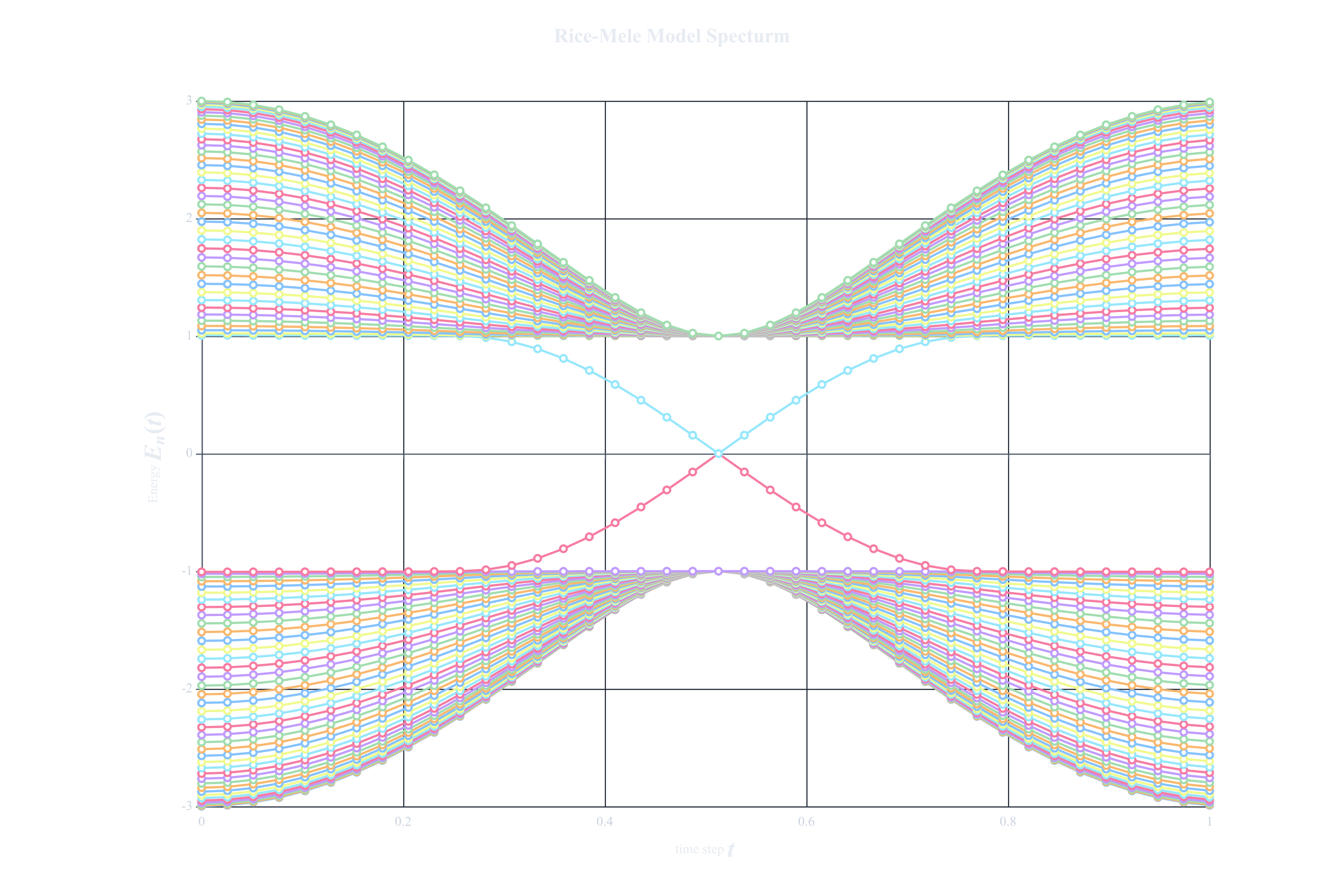
In the last line we save the figure in a directory called topological-physics and will save a the plot in a .figure file. When opening it in the workshop you should see the following plot below

.

We can now see that throughout the cycle we see that there is a crossing that occurs halfway. One eigenstate in the conduction band goes to the valence band, and vice-versa. All other states however remain in their respective bands.

What's Next?

• Write a function that can plot the eigenstates.
• Find a way to determine which eigenstates are edge modes. Plot them and show they are exponentially suppressed
• Plot the Pumping of one of the edge modes, visualize how edge modes move around through the cycle.
• Does disordering the $v,w,u$ change the physics? What about about other perturbations?
• Extend the static SSH Model to 2D, are there edge modes?

Documentation Contributors

Sebastien J Avakian