The Coulomb Operator

In this tutorial, we tackle a problem in device physics: characterizing the electronic structure of a Single-Electron Transistor (SET).

SETs are nanoscale devices where electrons tunnel one by one through a "quantum dot" island. Experimentally, one measures the conductance of the device while sweeping a gate voltage. This results in the famous "Coulomb Blockade" oscillations, where conductance is suppressed except at specific values of the gate voltage/chemical potential where sharp peaks appear.

These peaks correspond to resonance conditions where an electron can enter or leave the quantum dot. The position of these peaks allows us to map out the energy cost of adding electrons to the system. Specifically, the $N$-th peak occurs when the chemical potential of the leads matches the transition energy of the dot: $\mu(N) = E(N) - E(N-1)$ where $E(N)$ is the ground state energy of the system with $N$ electrons. The spacing between peaks tells us the addition energy, which is determined by both the quantum confinement (orbital energies) and the strong electrostatic repulsion between electrons.

To reproduce these experiments theoretically, our goal is to compute the ground state energies $E(N)$ for varying numbers of electrons. Because electron-electron interactions are crucial here, simple single-particle models are insufficient. We must solve the many-body Schrödinger equation.

The Physical Model

We model the quantum dot as a set of discrete single-particle orbitals (obtained, for example, from semi-classical simulations) occupied by electrons that interact via the Coulomb force.

The Hamiltonian governing this system is the Coulomb Hamiltonian. In second quantization, it is expressed in terms of creation ($a_i^\dagger$) and annihilation ($a_i$) operators:

$$H = \sum_{i} v_{i} a_i^\dagger a_i + \frac{1}{2} \sum_{i,j,k,l} V_{ijkl} a_i^\dagger a_j^\dagger a_k a_l$$

Here:

• $v_{i}$ represents the energy of orbital $i$ (including kinetic and potential energy).
• The last term is the Coulomb Operator, representing the two-body interaction.

The tensor $V_{ijkl}$ (often called Coulomb integrals or Coulomb tensor) encodes the strength of the repulsion between electrons in different spatial orbitals. It is calculated by integrating the Coulomb potential $\frac{e^2}{4\pi\epsilon_0 r_{12}}$ over the spatial wavefunctions $\phi(r)$ of the involved orbitals:

$$V_{ijkl} = \int \int \frac{e^2}{4\pi\epsilon_0 r_{12}} \phi_i^*(r_1) \phi_j^*(r_2) \phi_k(r_1) \phi_l(r_2) dr_1 dr_2$$

Construction and application of the corresponding operator is the most computationally demanding part of the problem.

In this tutorial, we will use Aleph to:

1. Construct this Hamiltonian effectively.
2. Compute the ground state energy $E(N)$ for different electron numbers.
3. Simulate the addition energy spectrum of the SET.

Building the Coulomb Hamiltonian

In this section, we will build the second quantized form of the Coulomb Hamiltonian step by step using Aleph. We assume that single-particle wavefunctions $\phi_i(r)$ are known from semi-classical device simulations and the Coulomb integrals $V_{ijkl}$ are provided.

We also assume the single-particle wavefunctions are spin-degenerate, meaning that each spatial orbital can be occupied by two electrons with opposite spins, and that the Coulomb integrals are spin-independent. This allows us to simplify the Hamiltonian by summing over spin indices, leading to a more compact representation of the Coulomb interaction. Our Hamiltonian can then be expressed as:

$$H = \sum_{i,\sigma} v_{i} a_{i,\sigma}^\dagger a_{i,\sigma} + \sum_{i,j,k,l,\sigma,\sigma'} V_{ijkl} a_{i\sigma}^\dagger a_{j\sigma}^\dagger a_{k\sigma} a_{l\sigma}$$

where $\sigma$ and $\sigma'$ represent the spin indices. The first term represents the single-particle energy contribution, while the second term captures the two-body interactions between electrons.

This is translated in Aleph as follows:

def make_full_hamiltonian(L, vi, vijkl){
    var H = operator_sum(as_real)
    for (var i=0; i < L; ++i) {
        H += vi[i/2] * Number(i)
    }
    for (i : [0..L]) {
        for (j : [0..L]) {
            for (k : [0..L]) {
                for (l : [0..L]) {
                    if(i % 2 != l % 2){
                        continue; // same spin
                    }
                    if(j % 2 != k % 2){
                        continue; // same spin
                    }
                    H += (0.5 * vijkl[i/2, j/2, k/2, l/2]) * (Create(i) * Create(j) * Destroy(k) * Destroy(l))
                }
            }
        }
    }
    return H
}

You may wonder why we divide by two in vi[i/2] and vijkl[i/2, j/2, k/2, l/2]. This is because we are summing over spin indices, and each spatial orbital can be occupied by two electrons with opposite spins. By dividing the index by two, we effectively account for the spin degeneracy in our Hamiltonian construction. Our convention here is that spin-up and spin-down states are indexed consecutively, so the spatial orbital index is obtained by integer division of the fermionic mode index by two.

We now have the Coulomb Hamiltonian in second quantized form, and we can use it to compute the ground state energy of the system. We can use quantum mechanics 101:

• Compute matrix elements of the Hamiltonian in a chosen basis.
• Assemble the Hamiltonian matrix;
• Diagonalize it to find the eigenvalues and eigenvectors.

These steps are achieved with simple calls to Aleph's linear algebra routines. The matrix function can be used to compute the matrix elements of the Hamiltonian in the computational basis, and the eigensolver function can be used to diagonalize the Hamiltonian matrix and find its eigenvalues and eigenvectors.

def diagonalize_full_hamiltonian(H){
    var Hmat = matrix(H, as_real)
    var results = eigensolver(Hmat, ["is_hermitian" : true])
    return results
}

var f = HDF5File("kothar.hdf5")
var vijkl = f.read("Coulomb", as_tensor | as_real)
var vi = f.read("Energies", as_matrix | as_real)
var v0 = vi[0]
vi /= v0
vijkl /= v0

var L = 6
var Hfull = make_full_hamiltonian(L, vi, vijkl)
var results = diagonalize_full_hamiltonian(Hfull)

A point to note is that we rescale the Coulomb integrals and the local potential by the same factor v0, which is the energy of the lowest single-particle orbital. This is a common practice to make the parameters dimensionless which can help with numerical stability. Indeed, the input data from the HDF5 file may be in Joules, and since we're dealing with microscopic scales the numbers can be in the 1e-20 - 1e-30 range, and rescaling them can prevent numerical issues during diagonalization.

After diagonalizing the Hamiltonian matrix, we obtain all eigenvalues. We need to do a bit more work to extract the ground state energy for given number of electrons, which is really what we want. Why? Because as we are sweeping the gate voltage, we are effectively changing the number of electrons in the system, and we want to track how the ground state energy changes with respect to the number of electrons. To do this, we can sort the eigenvalues and identify the lowest energy state for each electron number. This will allow us to construct a plot of ground state energy as a function of electron number, which can be directly compared to the experimental conductance peaks.

var N_electrons = 3
def filter_results(results, L, N){
    var vals = results.eigenvalues()
    var vecs = results.eigenvectors()
    var op = NumberN([0..L])
    var Nvals = []
    for (var i=0; i < size(vals); ++i) {
        var avg_n = expval(op, vecs.col(i))
        if (round(avg_n) == N){
            Nvals.push_back(vals[i])
        }
    }
    return Nvals
}

var eigenvalues = filter_results(results, L, N_electrons)
print(eigenvalues)
// [3.5304745766826, 3.5304745766826, 3.5304745766826, 3.53047457668261, 3.59084527688316, 3.59084527688316, ...

In the example above, we define a function filter_results that takes the eigenvalues and eigenvectors from the diagonalization, along with the system size L and the desired number of electrons N. We construct a number operator op that counts the total number of electrons in the system. We then loop through each eigenvector, compute the expectation value of the number operator, and check if it matches the desired electron number N. If it does, we add the corresponding eigenvalue to our list of filtered eigenvalues. This allows us to extract the ground state energy for a specific electron number, which is crucial for analyzing the conductance peaks in the single-electron transistor.

Symmetries of the Coulomb Hamiltonian

The previous procedure will do for small systems, but as the system size grows, the Hilbert space dimension grows exponentially, making it computationally infeasible to diagonalize the Hamiltonian directly. However, we can exploit symmetries of the Coulomb Hamiltonian to reduce the effective size of the Hilbert space and make the problem more tractable. The Coulomb Hamiltonian typically exhibits several symmetries, such as particle number conservation, spin conservation, and spatial symmetries. By identifying these symmetries, we can block-diagonalize the Hamiltonian into smaller subspaces, each corresponding to a specific symmetry sector.

In this tutorial, we show how to leverage particle number conservation. Beside the computational advantages, this also allows us to directly compute the ground state energy for a given number of electrons, which is what we are interested in when analyzing the conductance peaks in the single-electron transistor. By focusing on the relevant symmetry sectors, we can efficiently compute the ground state energies for different electron numbers and gain insights into the electronic structure of the system as a function of gate voltage.

The procedure for exploiting symmetries is as follows:

def diagonalize_hamiltonian(H, L, N)
{
    // We request few eigenvalues in this sector
    var nev = 6
    var dim = 1 << L
    var sym_state_vector = state_vector(as_fermion | as_number | as_real, ["num_sites" : L, "number" : N])
    var sym_opts = ["state_vector" : sym_state_vector, "is_hermitian" : true, "is_real" : true]
    var sym_results = iterative_eigensolver(H, dim, nev, sym_opts)
    return sym_results[0] // eigenvalues
}

var results = diagonalize_hamiltonian(Hfull, L, N_electrons)
print(results.list()[0])
// [3.5304745766826, 3.5304745766826, 3.5304745766826, 3.5304745766826, 3.59084527688316, 3.59084527688317] 

Comparing this with the full diagonalization results, we see that we get the same ground state energy for 3 electrons, but we are able to compute it without ever building the full Hamiltonian matrix. This is because our iterative eigensolver knows how to perform Hamiltonian-vector products directly with the operator. We are effectively diagonalizing a much smaller matrix corresponding to the symmetry sector with 3 electrons, rather than the full Hamiltonian matrix which includes all possible electron numbers. This allows us to efficiently compute the ground state energies for larger systems, which is crucial for making meaningful comparisons with experimental data from single-electron transistors.

note

For small systems, the full diagonalization can be faster than iterative diagonalization, but as the system size grows, exploiting symmetries with iterative diagonalization becomes essential. Matrix-free iterative methods not only become more efficient but also enable us to access larger system sizes that are otherwise intractable with full diagonalization. This is particularly important in the context of the Coulomb problem, where the Hilbert space dimension grows exponentially with the number of sites and electrons.

Comes in CoulombSum

At the end of the previous section, we had to write a lot of code to build the Coulomb Hamiltonian. This is because the Coulomb operator is a specific instance of a more general class of operators known as two-body interaction operators. To make it easier for users to work with such operators, Aleph provides a built-in operator called CoulombSum that encapsulates the functionality we implemented manually in the previous section.

def make_hamiltonian(L, vi, vijkl){
    var H = operator_sum(as_real)
    for (var i=0; i < L; ++i) {
        H += vi[i/2] * Number(i)
    }
    H += 0.5 * CoulombSum(vijkl)
    return H
}

The CoulombSum operator automatically handles the summation over orbitals and spin indices and ensures that the resulting operator is correctly symmetrized. By using CoulombSum, we can significantly simplify our code and reduce the likelihood of errors in implementing the two-body interaction term. This allows us to focus more on analyzing the results and less on the intricacies of building the Hamiltonian, making our workflow more efficient and streamlined when studying systems with Coulomb interactions.

There is another advantage to using CoulombSum beyond just code simplicity. Creating operators is not free, and neither are products with vectors which is the main bottleneck in iterative eigensolvers. When we get to large systems sizes, take 30 single-particle orbitals for example, the number of terms in the Coulomb operator can be on the order of millions (indeed there are on the order of $30^4 = 810000$ terms). Building this operator naively and performing matrix-vector products with it can be computationally expensive. To understand why, you need to think about what happens when you apply the operator to a state vector. The terms of a sum of operators multiply the state vector one by one, and the results are accumulated into an output vector. If we have millions of terms, this means we need to perform millions of operator applications and accumulations, which can be very time-consuming. To make things worse, in the present case, each term is a product of four fermionic operators: Create(i) * Create(j) * Destroy(k) * Destroy(l). When applying such a product to a state vector, we need to apply the first operator, then apply the second operator to the result, and so on. This means we have to process the entire state vector multiple times for each term, leading to a significant computational overhead.

Now, when we use CoulombSum, we are not explicitly constructing the full operator with all its terms. Instead, CoulombSum is implemented with efficient algorithms that take advantage of the structure of the Coulomb interaction, allowing for much faster matrix-vector products without explicitly constructing the full operator. This means that even for large systems, we can still efficiently compute ground state energies and other properties without being bogged down by the complexity of the Coulomb operator.

Let's make sure we're getting the same ground state energy with CoulombSum as we did with our manual implementation:

var Hcoulomb = make_hamiltonian(L, vi, vijkl)
var results_coulomb = diagonalize_hamiltonian(Hcoulomb, L, N_electrons)
print(results_coulomb.list()[0])
// [3.5304745766826, 3.5304745766826, 3.5304745766826, 3.5304745766826, 3.59084527688316, 3.59084527688317] 

As we can see, we get the same ground state energy for 3 electrons using CoulombSum as we did with our manual implementation. This confirms that CoulombSum is correctly capturing the physics of the Coulomb interaction while providing a much more efficient way to compute the ground state energies for larger systems.

Speed comparison

In this section, we look at the scaling of the computational time with respect to system size when using CoulombSum compared to a naive implementation of the Coulomb operator and full matrix representation. We will compare the time taken to compute the ground state energy for different system sizes using both approaches. We expect that as the system size increases, the time taken by the naive implementation will grow much more rapidly than the time taken by CoulombSum, demonstrating the efficiency of the latter.

def slice_tensor(L, coulomb){
    var N_orb = L / 2
    var vijkl = zero_tensor([N_orb, N_orb, N_orb, N_orb], as_real)
    for (i : [0..N_orb]) {
        for (j : [0..N_orb]) {
            for (k : [0..N_orb]) {
                for (l : [0..N_orb]) {
                    vijkl[i,j,k,l] = coulomb[i,j,k,l]
                }
            }
        }
    }
    return vijkl
}

// reload full data just in case
var f = HDF5File("kothar.hdf5")
var coulomb_full = f.read("Coulomb", as_tensor | as_real)
var vi_full = f.read("Energies", as_matrix | as_real) 
var v0 = vi_full[0]

var Nsites = [6, 8, 10, 12]
var Nel = [3]
for (L : Nsites){
    for (N : Nel){
        var vijkl = slice_tensor(L, coulomb_full)
        vijkl = vijkl / v0
        var vi = vi_full.slice([0], [L/2])
        vi /= v0

        var Hfull = make_full_hamiltonian(L, vi, vijkl)
        var H = make_hamiltonian(L, vi, vijkl)
        print("L : ${L}, N : ${N}")
        {
            var result = benchmark_for(bind(diagonalize_full_hamiltonian, Hfull), 1000)
            print(result)
        }
        {
            var result = benchmark_for(bind(diagonalize_hamiltonian, Hfull, L, N), 1000)
            print(result)
        }
        {
            var result = benchmark_for(bind(diagonalize_hamiltonian, H, L, N), 1000)
            print(result)
        }
    }
}

For illustration purposes, we obtain the following results:

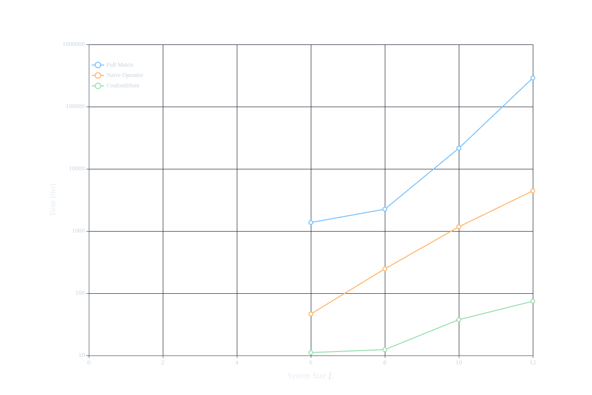
System Size (L)	Full Matrix	Naive Operator	CoulombSum
6	1.373 s	46.374 ms / 30x	11.139 ms / 123x
8	2.247 s	246.964 ms / 9x	12.438 ms / 181x
10	21.458 s	1.171 s / 18x	37.649 ms / 570x
12	4.814 min	4.432 s / 65x	74.500 ms / 3877x

From the results, we can see that as the system size increases, the time taken by the full matrix approach grows significantly, while the time taken by the naive operator implementation also grows but at a much slower rate. However, the CoulombSum implementation remains efficient even as the system size increases, demonstrating a much more favorable scaling compared to both the full matrix and naive operator approaches. This highlights the importance of using optimized implementations like CoulombSum when dealing with large systems in quantum mechanics.

The timings in the table are shown in the following figure:

Let's now focus on CoulombSum and bring the system size to the limit. We modify the loop above to run for larger system sizes and observe how the time taken scales. We expect that even for larger systems, CoulombSum will still be able to compute the ground state energies efficiently, while the full matrix approach would become infeasible due to memory constraints.

var Nsites = [8..61][::2]
var Nel = [4, 6, 8]
for (N : Nel){
    for (L : Nsites){
        var vijkl = make_tensor(L, coulomb)
        vijkl = vijkl / v0
        // var Hfull = make_full_hamiltonian(L, vi, vijkl)
        var H = make_hamiltonian(L, vi, vijkl)
        print("L : ${L}, N : ${N}")
        {
            var result = benchmark_for(bind(diagonalize_hamiltonian, H, L, N), 1000)
            print(result)
        }
    }
}

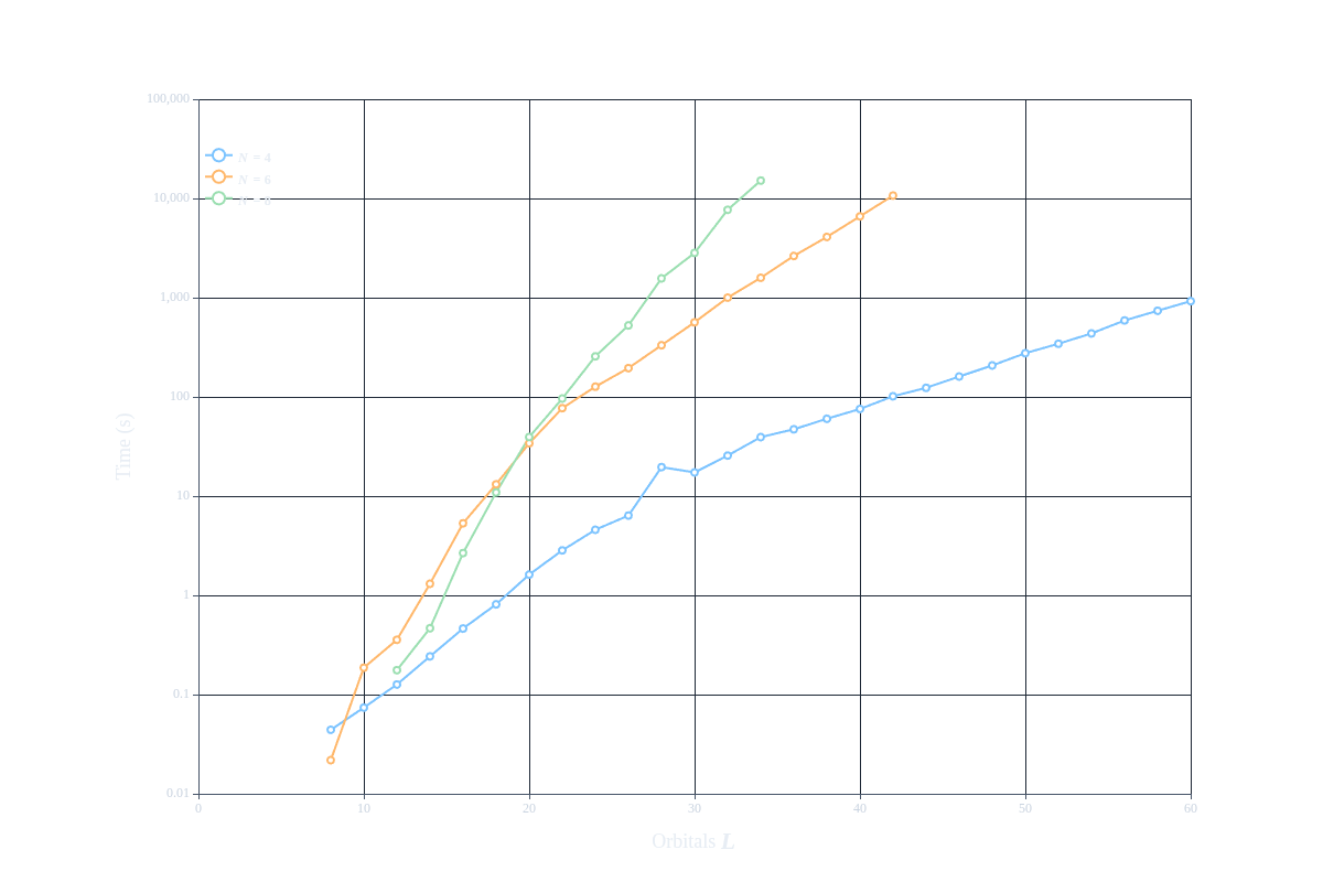
Using our 64 core machine (an AMD Ryzen Threadripper PRO 7985WX), we can reach system sizes up to 60 sites (30 spatial orbitals) and 8 electrons in a reasonable time frame (a few hours). This is a significant improvement compared to the full matrix approach, which would be completely infeasible for such large systems due to the exponential growth of the Hilbert space. The CoulombSum implementation allows us to efficiently compute ground state energies for larger systems, enabling us to study more realistic models of quantum dots and single-electron transistors. We report all timings in the table below:

System Size (L)	N=4	N=6	N=8
8	44.145 ms (~7e1)	21.818 ms (~3e1)	-
10	73.883 ms (~2e2)	186.525 ms (~2e2)	-
12	126.330 ms (~5e2)	356.333 ms (~9e2)	176.211 ms (~5e2)
14	242.527 ms (~1e3)	1.308 s (~3e3)	466.112 ms (~3e3)
16	462.950 ms (~2e3)	5.323 s (~8e3)	2.668 s (~1e4)
18	812.176 ms (~3e3)	13.152 s (~2e4)	10.882 s (~4e4)
20	1.619 s (~5e3)	34.110 s (~4e4)	39.393 s (~1e5)
22	2.840 s (~7e3)	1.283 min (~7e4)	1.604 min (~3e5)
24	4.581 s (~1e4)	2.113 min (~1e5)	4.271 min (~7e5)
26	6.366 s (~1e4)	3.250 min (~2e5)	8.757 min (~2e6)
28	19.597 s (~2e4)	5.525 min (~4e5)	26.072 min (~3e6)
30	17.325 s (~3e4)	9.406 min (~6e5)	47.075 min (~6e6)
32	25.614 s (~4e4)	16.668 min (~9e5)	2.133 h (~1e7)
34	39.322 s (~5e4)	26.417 min (~1e6)	4.204 h (~2e7)
36	47.139 s (~6e4)	43.859 min (~2e6)	-
38	1.003 min (~7e4)	1.137 h (~3e6)	-
40	1.259 min (~9e4)	1.832 h (~4e6)	-
42	1.691 min (~1e5)	2.970 h (~5e6)	-
44	2.057 min (~1e5)	-	-
46	2.674 min (~2e5)	-	-
48	3.459 min (~2e5)	-	-
50	4.594 min (~2e5)	-	-
52	5.720 min (~3e5)	-	-
54	7.267 min (~3e5)	-	-
56	9.820 min (~4e5)	-	-
58	12.304 min (~4e5)	-	-
60	15.371 min (~5e5)	-	-

The effective Hilbert space dimension for each combination of system size and electron number is also reported in the table above (in parentheses). We can see that even for large system sizes like 60 sites and 4 electrons, we are able to compute the ground state energy in a reasonable time frame, which would be completely infeasible with a full matrix approach. This demonstrates the power of using optimized implementations like CoulombSum when dealing with large systems in quantum mechanics.

The timings for the larger system sizes are shown in the following figure:

Putting it all together

In this section, we compute the charging energy spectrum of the single-electron transistor as a function of gate voltage using the tools we have acquired in the previous sections. We will compute the ground state energy for different electron numbers and extract the chemical potentials $\mu(N) = E(N) - E(N-1)$. The values of $\mu(N)$ correspond to the gate voltages where the $N$-th electron can enter the dot (conductance peaks). The difference between consecutive chemical potentials gives the addition energy $E_{add}(N) = \mu(N+1) - \mu(N)$, which tells us how much extra energy is needed to add one more electron due to Coulomb repulsion.

def get_model(L) {
    var f = HDF5File("kothar.hdf5")
    var coulomb_full = f.read("Coulomb", as_tensor | as_real)
    var vi_full = f.read("Energies", as_matrix | as_real) 
    var v0 = vi_full[0]

    var vijkl = slice_tensor(L, coulomb_full)
    vijkl /= v0
    var vi = vi_full.slice([0], [L/2])
    vi /= v0
    
    var H = make_hamiltonian(L, vi, vijkl)
    return Pair(H, v0)
}

var L = 10 
var model_data = get_model(L)
var H = model_data.first
var v0 = model_data.second
var JtoMev = 6.241509074461E+21 

var energies = []
var Nel = [0..L-1] // 0 to L electrons

print("Computing ground state energies...")
for (N : Nel){
    if (N == 0) {
        energies.push_back(0.0)
    } else if (N == 1){
        energies.push_back(1.0)
    } else {
        var results = diagonalize_hamiltonian(H, L, N)
        energies.push_back(results[0]) 
    }
}

print("Chemical Potentials (mu(N) = E(N) - E(N-1)) in meV:")
for (i : [1..size(energies)]) {
    var mu = (energies[i] - energies[i-1]) * v0 * JtoMev
    print("N=${i}: ${mu} meV")
}

print("Addition Energies (E_add(N) = mu(N+1) - mu(N)) in meV:")
for (i : [1..size(energies)-1]) {
     var E_add = (energies[i+1] - 2*energies[i] + energies[i-1]) * v0 * JtoMev
     print("N=${i}: ${E_add} meV")
}

The output reveals the shell structure of the quantum dot. We observe that addition energies are non-zero (manifestation of Coulomb blockade) and vary with $N$, reflecting the interplay between confinement energy and electron-electron interaction. Large peaks in addition energy would indicate particularly stable configurations (like filled shells).

Key takeaways

• Coulomb Operator Complexity: The Coulomb interaction involves four-fermion terms, leading to a number of terms scaling as $O(L^4)$.
• Efficient Implementation: Aleph's CoulombSum provides an optimized implementation for two-body interactions, significantly outperforming naive construction and full matrix representations, especially for large systems.
• Symmetries: Exploiting particle number conservation is crucial for reaching larger system sizes. It allows us to block-diagonalize the Hamiltonian and target specific charge states relevant for device physics.
• Iterative Solvers: Matrix-free iterative methods (like Lanczos/Arnoldi) are essential when the Hilbert space becomes too large to store in memory. They work seamlessly with Aleph's operator objects.

Recommended next steps

• Spin Symmetry: In this tutorial we only used particle number conservation. Try to extent the diagonalize_hamiltonian function to also target specific spin sectors ($S_z$) to further reduce computational cost.
• Disorder: Introduce random variations in the local potentials (vi) to simulate impurities in the quantum dot and study their effect on the addition energy spectrum.

References

1. Aleph Documentation: Refer to the official documentation for more details on CoulombSum, eigensolver, and symmetry handling.
2. Quantum Transport: Y. V. Nazarov and Y. M. Blanter, Quantum Transport: Introduction to Nanoscience, Cambridge University Press (2009).
3. Single-Electron Transistors: M. H. Devoret and R. J. Schoelkopf, Amplifying quantum signals with the single-electron transistor, Nature 406, 1039 (2000).