Free fermions

In this tutorial we use the quantum toolkit, specifically the operator framework and the free fermion features, to study the dynamics and eigenstates of a free fermion system. For a comprehensive introduction to free fermion systems and their representation, see the concept Non-interacting fermions.

note

In the context of non-interacting fermionic models, we make use of the word free as a shorthand for the single-particle sector, in analogy to a single fermionic particle free to roam in a potential landscape.

Below we will see how the free fermion features can be used to efficiently simulate and study the time evolution of a single fermion bouncing in a closed boxed containing a centered potential well. Furthermore, we will extract the eigenstates of the system and study their structure by analyzing the probability distribution of the particle. More precisely, we will:

• Study the dynamics of a free fermion initially confined to one edge of the box.
• Study the probability distribution of the ground-state and show that it is localized near the impurity.

First, we showcase how the problem can be solved with the operator_free functionalities. Second, we show how to dramatically increase the performance and system size by making use of free_stencil which exploits the structure of the problem.

Method 1: Using the operator_free factory

Constructing the Hamiltonian

We want to describe the dynamics of an electron that is free to move in a box with closed boundary conditions in the presence of an impurity. This can be done by first constructing a square lattice of size $L \times L$. In Aleph (see the Lattice tutorial for more details on how to use the lattice functionalities) we can construct a square lattice as follows

var L = 1000; // Specify the system size of LxL
var bcs = [boundary_condition.open, boundary_condition.open]
var square_lattice = lattice("square", [L,L], bcs); // Create the lattice

Next, we add nearest neighbor hopping terms at every site along both the $x$ and $y$ axis. The hopping terms capture the tendency of the electronic wave-function to delocalize in free space. The hopping Hamiltonian is given by

$$H_{\text{hopping}} = -\gamma\sum_{x=0,y=0}^{L-2}(c_{x,y}^{\dagger}c_{x+1,y} + c_{x,y}^{\dagger}c_{x,y+1}) + \text{h.c}$$

where $\gamma$ sets the energy scale of the hopping terms, chosen here to be $\gamma = 1$. In Aleph, we can construct the hopping hamiltonian as follows

var H_hopping = operator_sum(as_real) // Create an empty initial operator sum

// Create displacement vectors along the x and y direction
var delta_x = lattice_coordinate([1,0]);
var delta_y = lattice_coordinate([0,1]);
var gamma = 1.0;

// Go through every coordinate in the lattice
for (coord : lattice_range(square_lattice)) { 

    // Adding the hopping terms
    var x_coords = [coord, coord + delta_x]; // The coordinates [(x,y), (x+1,y)]
    var y_coords = [coord, coord + delta_y]; // The coordinates [(x,y), (x,y+1)]

    if (square_lattice.contains(coord + delta_x)) // Check if (x + 1, y) is in the lattice
    {
        // Convert the x hopping coordinates to the corresponding matrix indices
        var x_indices = [square_lattice.to_index(x_coords[0]), square_lattice.to_index(x_coords[1])]

        H_hopping += -1.0*gamma*Hop(x_indices);
    }

    if (square_lattice.contains(coord + delta_y)) // Check if (x, y + 1) is in the lattice
    {
        // Convert the y hopping coordinates to the corresponding matrix indices
        var y_indices = [square_lattice.to_index(y_coords[0]), square_lattice.to_index(y_coords[1])]

        H_hopping += -1.0*gamma*Hop(y_indices);
    }
}

Additionally, we add an impurity at the center of the lattice in the form of a Gaussian potential well

$$H_{\text{impurity}} = U_{\text{center}}\sum_{x=0,y=0}^{L-1} e^{-\frac{1}{2\sigma^2}(( x - \mu_x)^2 + (y - \mu_y)^2)}(n_{x,y})$$

where $\sigma = L/4$ sets the width of the potential well, $U_{\text{center}} = -6\gamma = -6$ is its maximum depth and $(\mu_x, \mu_y)$ is the position around which it is centered, chosen here to be $(\mu_x, \mu_y) = (L/2,L/2)$.

note

The parameter $\sigma$ is best chosen when used to approximate the surface area that contains the potential well. For a lattice of size $L \times L$ for which the lattice spacing is set to $1$, then the potential well approximately occupies a fraction $\sigma^2/L^2$ of the total surface area. Hence the choice $\sigma = L/4$ implies the potential well occupies about $1/16$ of the total system.

In Aleph, we can construct the impurity Hamiltonian as follows:

var H_impurity = operator_sum(as_real) // Create an empty initial operator sum
var U_center = -6.0
var sigma = L/4.0
var mu_x = (L-1)/2.0  // (L-1) to account for zero indexing
var mu_y = (L-1)/2.0

// Go through every coordinate in the lattice
for (coord : lattice_range(square_lattice)) { 

    var x_site = coord.primitive_vector()[0];
    var y_site = coord.primitive_vector()[1];
    var local_amplitude = U_center*exp(-(1.0/(2.0*sigma**2))*((x_site - mu_x)**2 + (y_site - mu_y)**2));
        
    // Get the corresponding matrix index 
    var n_index = square_lattice.to_index(coord)
    H_impurity += Number(n_index)*local_amplitude;
}

// Construct the total Hamiltonian
var H_tot = H_hopping + H_impurity

where the last line constructs the Hamiltonian of the system

$$H_{\text{tot}} = H_{\text{hopping}} + H_{\text{impurity}}$$

In its current form, the obtained Hamiltonian has not been restricted to the single-particle sector, and so by default will expect to interact with state vectors of size $2^L$. Given our goal we would like to cast the obtained Hamiltonian to its free representation, which can be achieved by making use of the operator_free factory, which returns an operator representing the free matrix representation of the operator (see the concept Non-interacting fermions for more details).

//First specify the options needed to build a free operator
var free_option = as_fermion | as_singleparticle

//Extract the operator representation
var free_operator = operator_free(H_tot, free_option)

If the explicit internally stored matrix is desired instead, it can be easily obtained by making use of the matrix factory with the appropriate options.

//Extract the bare free matrix representation
var free_matrix = matrix(H_tot, free_option)

note

The choice of constructing either a matrix or an operator depends on the problem at hand. The matrix factory returns a matrix which gives the user a lot of control over the data at the cost of having to ensure that custom made interactions with other objects behave as intended. Making use of operator_free produces an operator which comes with specialized methods, safety checks and optimizations at the cost of loosing precise control over how it interacts with other objects.

Studying the dynamics

Now that we have constructed the Hamiltonian, our next task is to study the time evolution of a state initially localized to one edge of the system. Here we may do so by concentrating the weight of the electronic probability distribution uniformly on the top edge of the box.

$$\vert \psi(t = 0) \rangle = \frac{1}{\sqrt{L}}\sum_{x = 0}^{L-1}c_{x,0}^{\dagger}\ket{0}$$

In Aleph, we may achieve this as follows

//Create a single particle state
var free_state = state_vector(L**2, as_fermion | as_singleparticle); // The fermionic particle can occupy L**2 possible sites

var initial_coord = lattice_coordinate([0,0])
for (var x_pos = 0; x_pos < L; ++x_pos) //Loop over all the lattice coordinates
{ 
    var coord = lattice_coordinate([x_pos,0])
    var vector_index = square_lattice.to_index(coord);
    free_state[vector_index] = 1.0;
}
//Normalize the state
free_state.normalize()

Next, we want to time-evolve the electronic wave function in time. From the solution to the time-independent Schrödinger equation, we have that

$$\ket{\psi(t = T)} = e^{-iH_{\text{tot}}T}\ket{\psi(0)} = (e^{-iH_{\text{tot}}(T/N_{T})})^{N_{T}}\ket{\psi(0)} = U_{dT}^{N_{T}}\ket{\psi(0)}$$

where $U_{dT} = e^{-iH_{\text{tot}}dT}$, $dT = T/N_{T}$ and $T$ is the total time for which we want to evolve the system. We have also introduced $N_{T}$ which is the total number of time steps we would like to take between $t = 0$ and $t = T$ to study how the wave function evolves in time. As can be observed from the equation above, this can be achieved by applying the unitary $U_{dT}$ repetitively on the initial state $\ket{\psi(0)}$. To do so, we first construct the unitary $U_{dT}$ and then apply it recursively on the state. We could construct the explicit matrix exponential to preform this task, but a much faster method makes use of operator_function which leverages efficient Krylov methods to accelerate the calculation of matrix on vector multiplications. Crucially it avoids the explicit calculation of the matrix exponential. (see the Krylov evolution and operator matrix tutorial for more details on how to use Krylov methods)

//Setup
var T = 20.0
var N_T = 200
var dT = T/N_T
var vector_size = L**2

// Krylov setup
var func = fun[dT](x) { return exp(-1i * dT * x) } // Specify the function that generates the unitary matrix
var Nkrylov = 4

// Construct an operator function
var U_dT = operator_function(free_operator, vector_size ,func, ["krylov_dimension" : Nkrylov])
var free_coefficients = free_state.coefficients()
for (var time = 0; time < N_T; ++time){
    U_dT >> free_coefficients
}

note

Performing time evolution by making use of the first method will in general be more precise, but it can be orders of magnitude slower than the second method. The appropriate choice is determined by the error tolerance for the problem at hand which is left to the discretion of the user.

The following animation displays the obtained probability distribution of finding the electron on any site of the lattice as a function of time. We see that the attractive impurity initially focuses the incoming probability distribution near the center. Then, the particle scatters off the potential well. Some of the probability distribution is transmitted whilst some of it is reflected. Interestingly the reflected part of the probability distribution is concentrated around the $x = L/2$ axis, showing that an impurity can act as a sort of quantum lens.

Time evolution

Eigenmode analysis

As a final task in this tutorial, we study the ground state of the single-particle Hamiltonian $H_{\text{tot}}$. The ground state of $H_{\text{tot}}$ is the eigenstate of $H_{\text{tot}}$ with the smallest possible eigenvalue. It can be found by making use of the iterative_eigensolver as follows in Aleph (see the ground-state tutorial for more details on how to use Krylov methods)

var num_eigenpairs = 5
var eigen_pairs = iterative_eigensolver(free_matrix, num_eigenpairs)
var ground_state = eigen_pairs[1][0:L**2,0:1]
var excited_state = eigen_pairs[1][0:L**2,4:5]

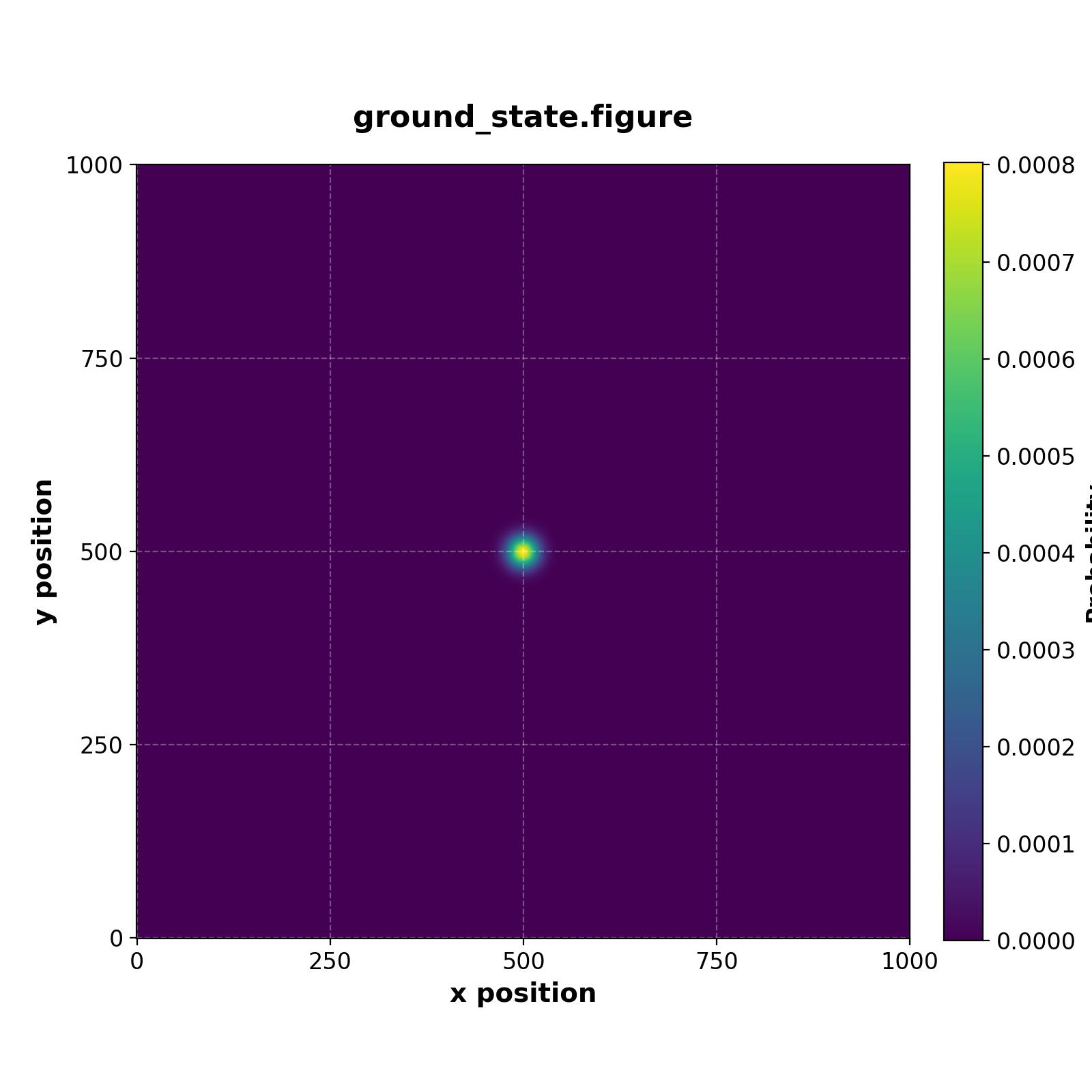
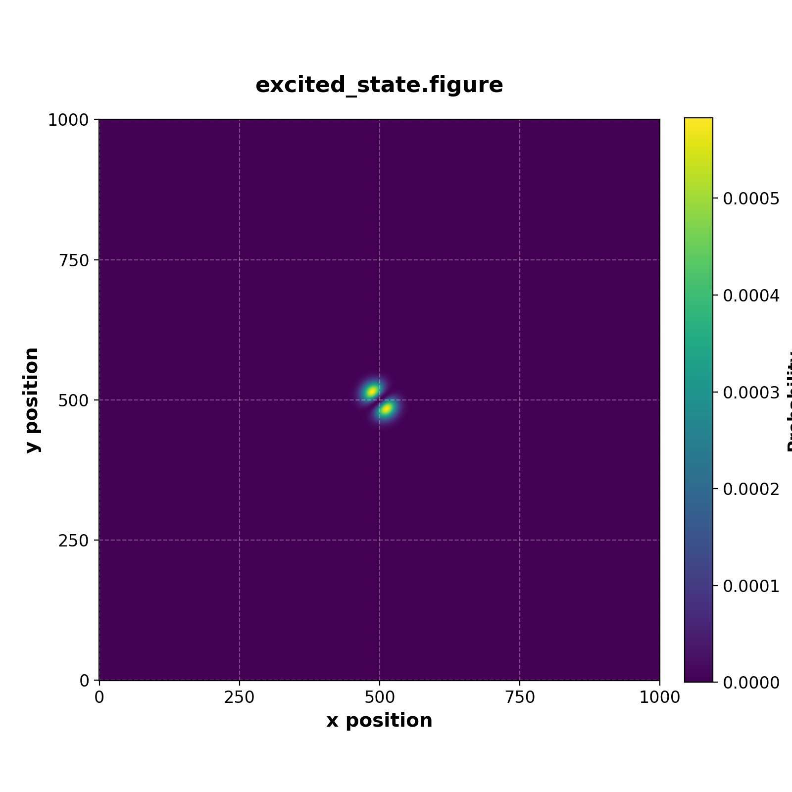
The following figures display the obtained probability distribution of finding the electron on any site of the lattice for the ground state and the fifth excited stationary state. We see that the ground-state is localized around the center as expected. The fifth excited stationary state exhibits four symmetrically opposite regions of high probability. These are reminiscent of the well-known electronic orbitals of the Hydrogen atom. We also observe regions for which the probability distribution vanishes. This fits the well-known fact that high energy solutions of the Schrödinger equation have an increasingly larger number of nodes as the energy increases.

Ground state	Fifth excited state

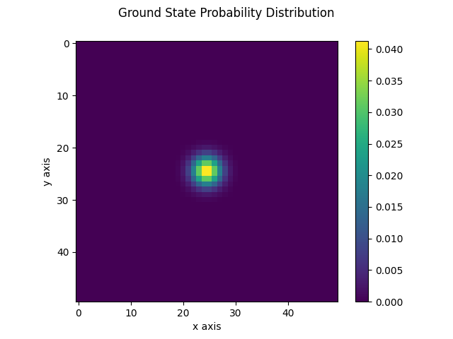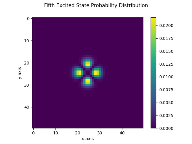Method 2: Solving with operator_stencil methods

The problem at hand contains a lot of redundancy that can be exploited to solve the problem in a time that is orders of magnitude faster than more naive method. For instance, the hopping terms of the Hamiltonian are repeated uniformly across the entire lattice and the Gaussian impurity potential is diagonal in the Fock basis. Combining these facts we can solve the problem as follows.

As before, we create a lattice, but this time we are more ambitious and specify a system size $L = 1000$

var L = 1000; // Specify the system size 10^6
var bcs = [boundary_condition.open, boundary_condition.open]
var square_lattice = lattice("square", [L,L], bcs); // Create the lattice

var U_center = -0.8
var sigma = L/4.0
var mu_x = (L-1)/2.0  // (L-1) to account for zero indexing
var mu_y = (L-1)/2.0

Next, we create a sparse diagonal matrix representing the potential generated by the Gaussian impurity

// Create the number potential
var size = L**2
var free_state = state_vector(size, as_fermion | as_singleparticle);
var number_mat =  identity([size, size], as_real | as_sparsematrix)
var index_positions = uninitialized([size], as_array | as_integer)
var values = uninitialized([size], as_real | as_array)

To construct the state we this time opt instead for a state exponentially localized on the left edge. We get

for (var x_site = 0; x_site < L; ++x_site) { 
    for (var y_site = 0; y_site < L; ++y_site) { 
        var index = x_site + L*y_site
        var local_amplitude = U_center*exp(-(1.0/(2.0*sigma**2))*((x_site - mu_x)**2 + (y_site - mu_y)**2));
        index_positions[index] = index
        values[index] = local_amplitude
        free_state[index] = exp(-(20*x_site)/(L)) // Stale localized on the edge
    }
}
number_mat.insert(index_positions,index_positions,values)
free_state.normalize()

Then we make use of the operator_stencil factory which exploits repeated structure of the hopping terms. To build a stencil, we specify its corresponding displacements vectors, the dimensions of the lattice, the values of the stencil and the boundary conditions. We get

var displacements = [[-1,0],[1,0],[0,1],[0,-1]]
var dimensions = [L,L] 
var stencil_values = [-1.0,-1.0,-1.0,-1.0] 
var boundary_conditions = [boundary_condition.open, boundary_condition.open]
var h_hop = operator_stencil(["displacements":displacements,"dimensions":dimensions,"values":stencil_values,"boundary_conditions":boundary_conditions])

Finally, we construct the total Hamiltonian by taking the sum and perform the time evolution by making use of operator_function to avoid the explicit calculation of the matrix exponential.

//Construct the sum
var h_tot = h_hop + operator_free(number_mat, as_real)
//Generate corresponding time evolution operator
var U_dt = operator_function(h_tot, size, func, ["krylov_dimension" : N_krylov])

//Time evolve
for (var t = 0; t < tot_time; ++t){
    U_dt >> free_state
}

The resulting vector can be saved at every time step, whose data can be used to construct an animation of the time evolution.

Time evolution

We can also extract the first and second excited state by calling iterative_eigensolver as follows

// Get the ground state
var num_eigenpairs = 2
var eigen_pairs = iterative_eigensolver(h_tot, size, num_eigenpairs)
var ground_state = eigen_pairs[1][0:L**2,0:1]
save(ground_state, "ground_state.figure")
var excited_state = eigen_pairs[1][0:L**2,1:2]
save(excited_state, "excited_state.figure")

Which generates the figures

Ground state	Fifth excited state

What's next?

• Can this be used to study the energy levels of the hydrogen atom? What would need to be changed?
• Which time evolution method is faster? Which is more precise? What is the minimum Krylov subspace dimension needed before the state start to diverge from one another?
• What happens when we add more impurities? Change the sign of $U_{\text{center}}$?

Documentation Contributors

Pierre-Gabriel Rozon