Stochastic Series Expansion

This tutorial explains how to use Aleph's stochastic series expansion (SSE) Monte Carlo API.

Formalism

The stochastic series expansion (SSE) is a Markov chain Monte Carlo formalism that is well suited to estimating expectation values of quantum systems that are in thermal equilibrium with a bath of inverse temperature $\beta$. In this section we develop the formalism of the stochastic series expansion and fix some terms and conventions before demonstrating how the formalism is implemented in Aleph.

The SSE starts from the partition function,

$$\mathcal{Z} = \text{Tr}\left(e^{-\beta\hat{H}}\right)$$

where,

$$\hat{H} = \sum_{s,\alpha} \hat{h}_{s,\alpha}$$

is a Hamiltonian with terms acting on sites collectively labelled by $s$. The index $\alpha$ represents a particular decomposition of the terms into non-branching operators. The first step is to perform a Taylor series expansion of the partition function,

$$\mathcal{Z} = \sum_{n=0}^{\infty}\frac{\beta^n}{n!}\text{Tr}\left((-\hat{H})^n\right).$$

The exponentiated Hamiltonian inside the trace will result in terms that contain all possible orderings of product of the terms in the Hamiltonian. This still leaves us the task of evaluating the trace, which is exponentially difficult. The key step in the SSE to avoid this difficulty is to sample over a local basis, whose elements are non-branching with respect to the our choice of decomposition of the Hamiltonian. Explicitly,

$$\mathcal{Z} = \sum_{n=0}^{\infty}\sum_{\ket{b}}\frac{\beta^n}{n!}\bra{b}(-\hat{H})^n\ket{b}$$

where,

$$\hat{H}_{s,\alpha}\ket{b} \propto \ket{a'}, \quad \forall \,s,\,\alpha,\,\ket{b}.$$

Matrix elements, $\bra{b}\hat{h}_{s,\alpha}\ket{a'}$ are referred to as vertices, and are defined by the sites on which they act, and their input and output states (vertices with identical input and output are generally grouped together), and their magnitudes, or weights. Vertices can be given an additional attribute in the cluster variant of the SSE known as branch groups.

The no-branching condition allows us to efficiently sample over the powers of the Hamiltonian by introducing the concept of an operator string. We first fix an expansion cutoff $M$, which is determined during the equilibration phase of the Monte Carlo. The operator string is then defined as a product of length $M$ whose factors are either the identity matrix or one of the terms in the Hamiltonian. The operator string can the be written as $\sigma = (s_1,\alpha_1)(s_2,\alpha_2)\ldots(s_M,\alpha_M)$, where $\alpha=-1$ corresponds to the identity (in this case $s$ is taken to be all the sites). The number of non-identity terms corresponds to the expansion order of the operator string in the Taylor series. Because of the introduction of the identity in the operator string, we will over count the terms in the original expansion and must divide by the combinatorial factor. Thus we arrive at,

$$\mathcal{Z} = \sum_{n=0}^M\sum_{\ket{b}}\sum_{\sigma}\frac{\beta^n(M-n)!}{M!} \bra{b} \prod_{j=1}^M\hat{h}_{s_j,\alpha_j}\ket{b}.$$

Within this formalism, a variety of estimators are possible. The most efficiently estimated quantities are those that depend on the expansion order, such as the specific heat or energy. The second most efficiently estimated are those estimators that can be easily expressed as functions of the operator strings, such as operators that are diagonal in the computational basis, or the average value of terms in the Hamiltonian.

warning

An essential limitation of the SSE is that the weights of the vertices must all be positive, with lowest energy weights have the highest value. In the following examples, we demonstrate how this can be attained for the Heisenberg and Ising models. Discovering transformations that allow for sign-problem free simulation is still an active area of research.

The Antiferromagnetic Heisenberg Model (Abstract Loop Update)

The Heisenberg model is the essential model in the study of quantum magnetism, and its properties on various geometries and those of its extensions remain an active area of research interest. In this tutorial we show how to build an SSE for the Heisenberg model using aleph's framework. Before we can begin this process we need to do some work on the form of the Heisenberg Hamiltonian,

$$\hat{H} = \sum_{j,k} \vec{S}_j\cdot\vec{S}_k.$$

Defining a Geometry

The main object in the SSE framework is the SSEAlgorithm, which manages the simulation and records past configurations. We being by Constructing a lattice with neighbourhood rule(s), and an inverse temperature beta:

var LC = lattice_coordinate
var size = 6
var beta = 32.0

var alg = sse_algorithm(
    lattice("chain", [size], ["open"]),
    neighbourhood_rule("nn", LC([1])),
    beta
)

The neighbourhood rules correspond to the collections of sites on which terms in the Hamiltonian act, and are discussed in more detail here.

Adding Vertices

Now we have to specify the vertices that are added and removed from the operator string. First we can rewrite the Hamiltonian in terms of raising and lowering operators so that, with respect to the $z$ basis, the terms are non-branching,

$$\hat{H} = \sum_{j,k} \hat{S}_j^z \hat{S}_k^z + \frac{1}{2}(\hat{S}^+_j\hat{S}^-_k + \hat{S}^-_j\hat{S}^+_k)$$

Focusing first on the diagonal terms, we can see that the antiferromagnetic elements will have a weight of,

$$\bra{\uparrow\downarrow}\hat{S}^z_j\hat{S}^z_k\ket{\uparrow\downarrow} = \bra{\downarrow\uparrow}\hat{S}^z_j\hat{S}^z_k\ket{\downarrow\uparrow} = -\frac{1}{4}$$

while the ferromagnetic weights will be,

$$\bra{\uparrow\uparrow}\hat{S}^z_j\hat{S}^z_k\ket{\uparrow\uparrow} = \bra{\downarrow\downarrow}\hat{S}^z_j\hat{S}^z_k\ket{\downarrow\downarrow} = \frac{1}{4}$$

For the purpose of sampling we want the weights of the anti-ferromagnetic states to be greatest. We can achieve this by multiplying the Hamiltonian by $-1$ and shifting each local term by $\frac{1}{4}$,

$$\hat{H} \rightarrow \frac{1}{4}N_s - \hat{H}$$

where $N_s$ is the number of neighbourhoods.

warning

When estimating the energy in the SSE, we must remember to undo any shifts or scalings that we performed at this step.

This transformation introduces an additional problem: the off-diagonal weights are now negative. As long as the lattice is bipartite, we can perform a rotation about the $Z$ axis by $\pi$ and thus eliminate the negative sign. Denoting the shifted and scaled diagonal vertices with $\hat{h}_{s,1}$ and off-diagonal vertices with $\hat{h}_{s,2}$, we now have,

$$\bra{\uparrow\downarrow}\hat{h}_{s,1}\ket{\uparrow\downarrow} = \bra{\downarrow\uparrow}\hat{h}_{s,1}\ket{\downarrow\uparrow} = \frac{1}{4} \\ \\ \bra{\uparrow\downarrow}\hat{h}_{s,2}\ket{\downarrow\uparrow} = \bra{\downarrow\uparrow}\hat{h}_{s,2}\ket{\uparrow\downarrow} = \frac{1}{4}$$

The above vertices are often conveniently represented graphically. For example, the vertex $\bra{\uparrow\downarrow}\hat{h}_{s,1}\ket{\uparrow\downarrow}$

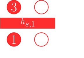
where solid red means spin up and the empty red circles are spin down.

Input and output states of the vertex are referred to as legs, and are numbered conventionally as shown above.

Now that we've transformed the Hamiltonian into a form with only positive weights we can add the vertices to the algorithm:

alg.add(sse_vertex([2, 2], [0, 1]), ["weights" : ["nn" : 0.5]])
alg.add(sse_vertex([2, 2], [1, 0]), ["weights" : ["nn" : 0.5]])
alg.add(sse_vertex([2, 2], [0, 1], [1, 0]), ["weights" : ["nn" : 0.5]])
alg.add(sse_vertex([2, 2], [1, 0], [0, 1]), ["weights" : ["nn" : 0.5]])

In the sse_vertex constructor, the first entries refer to the local dimensions of the legs, with the next entry referring to the input state for the vertex. If no output legs are specified, it's assumed that the outputs are identical to the inputs. Finally, a list of weights on each neighbourhood is required.

Initializing the State and Loop Update

We need to start off the SSE in particular state. This can be achieve by passing the initial state to the SSE via,

alg.initialize(Qbit(size), ["actions" : [1]])

note

The SSE can be initialized with any basis state, not just qubit states.

This function also initializes the abstract loop update, a non-local updating scheme for the SSE. By default, the algorithm is initialized with a single spin flip action, and a heat bath algorithm is used to ensure detailed balance.

How do we know that a loop update would work here? Looking at the vertices we can see that it's possible to transform any vertex into any other vertex by flipping two spins at a time. For example,

Such an update can be conceptualized as a worm that enters on one leg and exits on another, flipping the spins at each point. Because the trace is periodic, the worm must close on itself or terminate at an untraced site for the update to be valid.

The specific mechanics of the loop update are handled by SSEAlgorithm. Users can customize the probabilities and transformation types (suitable for higher spins and bosons) using the scattering_table described below.

If one wants to us a loop update, the initialize method supports the following options,

• scattering_update ("heat_bath_conservative"; legacy alias "heatbath_conservative")
• scattering_table
• untraced_sites

Equilibration

Markov chain Monte Carlo requires an equilibration period before the limiting distribution (in this case the partition function) is sampled. During the period, the expansion cutoff is allowed to vary.

var equil_steps = 4096
alg.equilibrate(equil_steps)

We could choose to record the configurations during this process, but configurations we observe would not be reflective of the equilbrium distribution. The amount of equilibration required depends on the system. Once the expansion cutoff is no longer increasing we can assume that the system has equilibrated.

Running the Simulation and Estimating the Order

At this point we can run the simulation and begin recording data. Aleph comes equipped with an estimator for the order that can be used to estimate the energy and specific heat.

var bin_size = 2048
var order_first_moment = sse_order_estimator([1,2], accumulator("binning", ["bin_size" : 2048]))

where the first argument determines the moments of the order to be estimated (for the specific heat we need both the first and second moments). The analytical formulae for the energy and specific heat can be derived from the SSE formalism above, and are given as functions of the average expansion order of the operator string,

$$E = -\frac{1}{\beta}\langle n \rangle, \\ C = \langle n^2 \rangle - \langle n \rangle - \langle n \rangle^2.$$

In practice, the bin_size should be set to be approximately the auto-correlation length. There are numerous ways to estimate auto-correlation lengths in the SSE. Aleph provides a logarithmic binning accumulator for this purpose. For this tutorial we select a length of 2048.

var nbins = 32 // a common choice
var simul_steps = nbins * bin_size 
alg.run(simul_steps, order, ["estimate_period" : 1, "record_period" : 1])

In the above we've also set the record period to $1$. This will record the operator string after each sweep and allow us to construct any other estimators we want.

Both run and equilibrate support the following options:

• flip_probability
• estimate_period (> 0)
• record_period (> 0)
• max_loop

Computing the Energy and Specific Heat

The order estimator will accumulate the values of the order during the simulation. We can then estimate the energy by supplying the shift and scaling that we initially applied to the Hamiltonian,

var energy = sse_energy(order, -1.0, 0.25 * (size - 1), beta)
var cv = sse_specific_heat(order)

Notice that the specific heat doesn't require the shift and scaling, as it is a function of the spectral statistics and therefore independent of such overall changes.

Diagonal Estimators and History

Any estimator that is diagonal in the simulation basis can be recovered using the history of the simulation, recorded during the run phase,

var history = alg.history()
var opstr = history[0]

var cutoff = opstr.cutoff()
var order = opstr.order()
var entries = opstr.data()

var e0 = entries[0]
print(to_string(e0))
print(e0.diagonal(), e0.vertex_id(), e0.support_id(), e0.sites())

Each entry contains the vertex index, the sites on which the vertex acts, the kind of support, and whether the vertex is diagonal. The history is given in terms of the vertex index on each slice, and there requires the user to reconstruct a compatible state from the history and vertex table if they want to write the full configuration.

Save and load algorithms via HDF5

var file = HDF5File("sse_algorithm_hdf5.h5", "w")
file.write("/my_simulation", alg)
file.write("/parent/my_simulation", alg)

var loaded_a = file.sse_algorithm("/my_simulation")
var loaded_b = file.sse_algorithm("parent/my_simulation")

Custom Loop Updates (Scattering Table)

By default, loop updates are constructed by attempted to flip both the entrance and exit spins by one, and the relative probability of selecting an exit flip based on the entrance leg is determined by the heat bath algorithm to ensure detailed balance.

Advanced users may want to implement more optimized loop scattering probabilities. This can be done by passing a scattering table directly to the initializer using the option "scattering_table". The table must be indexed by [vertex_id][support_id][action_id][entrance_leg][exit_leg] and the entries must contain,

• The cumulative probability of exiting on the given leg,
• An index corresponding to the new action type after the scatter,
• The new vertex index.
• A boolean indicating whether the new vertex is diagonal.

The Transverse Field Ising Model (Cluster Update)

The Transverse Field Ising Model (TFIM) is another paradigmatic model of quantum magnetism, and also represents a different flavour of stochastic series expansion update, namely the cluster update. The model in this case is given by,

$$\hat{H} = -\sum_{j, k} \hat{\sigma}^z_j \hat{\sigma}^z_k - h\sum_j \hat{\sigma}^x_j$$

We can define this model analogously to the Heisenberg model via,

var LC = lattice_coordinate
var size = 6
var beta = 32.0
var h = 0.2

var alg = sse_algorithm(
    lattice("chain", [size], ["open"]),
    [neighbourhood_rule("nn", LC([1])),
    neighbourhood_rule("onsite", LC([]))],
    beta
)

Notice that now we add the onsite neighbourhood rule for the transverse field term.

Like in the case of the Heisenberg SSE we can rescale and add a constant to ensure that the lowest energy matrix elements have the highest weights giving the terms,

$$\hat{h}_{s,0} = h \\ \hat{h}_{s,1} = h(\hat{\sigma}^+_s + \hat{\sigma}^-_s) \\ \hat{h}_{s,2} = (\hat{\sigma}^z\hat{\sigma}^z + 1)$$

The vertices are then,

$$\bra{\uparrow}\hat{h}_{s,1}\ket{\downarrow} = \bra{\downarrow}\hat{h}_{s,1}\ket{\uparrow} = h \\ \bra{\uparrow}\hat{h}_{s,0}\ket{\uparrow} = \bra{\downarrow}\hat{h}_{s,0}\ket{\downarrow} = h$$

and,

$$\bra{\uparrow\uparrow}\hat{h}_{s,2}\ket{\uparrow\uparrow} = \bra{\downarrow\downarrow}\hat{h}_{s,2}\ket{\downarrow\downarrow} = 2$$

Notice that an update that moves between these vertices would involve simultaneously flipping blocks of spins. In particular, for the two site vertex, it would involve flipping the spin on both the input and output legs. This type of model therefore requires a cluster update, where the legs of vertices are grouped into branches that can be transformed simultaneously according to a rule.

Vertices with Branch Groups

alg.add(
    sse_vertex([2, 2], [1, 1]),
    ["weights" : ["nn" : 2.0], "branch_groups" : ["nn" : [[0, 1, 2, 3]]]]
)
alg.add(
    sse_vertex([2, 2], [0, 0]),
    ["weights" : ["nn" : 2.0], "branch_groups" : ["nn" : [[0, 1, 2, 3]]]]
)
alg.add(
    sse_vertex([2, 2], [0]),
    ["weights" : ["onsite" : h], "branch_groups" : ["onsite" : [[0], [1]]]]
)
alg.add(
    sse_vertex([2, 2], [1]),
    ["weights" : ["onsite" : h], "branch_groups" : ["onsite" : [[0], [1]]]]
)
alg.add(
    sse_vertex([2, 2], [1], [0]),
    ["weights" : ["onsite" : h], "branch_groups" : ["onsite" : [[0], [1]]]]
)
alg.add(
    sse_vertex([2, 2], [0], [1]),
    ["weights" : ["onsite" : h], "branch_groups" : ["onsite" : [[0], [1]]]]
)

In the above example, notice that branch_groups must be paired with weights. Moreover, the branch groups determine which groups of spins can be transformed together.

Initializing the Simulation

Just like with the loop update, we can pass an option to the initializer to indicate how the branch groups should be transformed. The algorithm contains one named transformation suitable for spin-half models called "spinHalfFlip", which flips all the spins in the branch group. In this simulation we'll also demonstrate how to extract the reduced density matrix by excluding certain sites from the trace,

alg.initialize(Qbit(size), ["branching_update" : "spinHalfFlip", "untraced_sites" : [0, 1]])

Custom Cluster Updates (Branching Table)

Alternatively, users can provide a table directly to the initializer. This table has the following indices: [vertex_id][cluster_id][neighbourhood_id][branch_id] and contains a list with the following elements:

• The ratio of the logarithms of the weights of the vertices before and after the flip.
• The new vertex index.
• A boolean indicating whether the new vertex is diagonal.

Running and equilibrating the simulation follows the same steps as in the Heisenberg example above, with an additional option,

• flip_probability which determines the probability of flipping a cluster. Since all possible clusters are always constructed, it would leave the simulation invariant if they were all flipped with probability one. The default flip_probability is 0.5, which seems to work well.

Running the Simulation

Once again we can run and equilibrate the simulation,

var equil_steps = 4096
alg.equilibrate(equil_steps)

var simul_steps = 2**13
alg.run(simul_steps, ["estimate_rdm" : true, "estimate_period" : 1])

Notice that we've omitted the order estimator since we won't be needing it in this case. The simulation will now count the number of times each basis state appears on the untraced sites and store it in the count_matrix,

var count_matrix = alg.count_matrix()

The user can then normalize these entries to extract an estimate for the density matrix.

warning

The reduced density matrix is only estimated if the estimate_rdm boolean is passed as true.

Common validation errors to avoid

• Unknown keys in add, initialize, equilibrate, or run payloads.
• branch_groups without weights in add.
• Loop init without non-empty actions.
• Mixing loop and cluster initialization options.
• Unsupported scattering_update or branching_update.
• record_period or estimate_period set to 0.

Contributors

James Lambert