Mid-spectrum calculations with Chebyshev filters

The eigenspectrum of a Hamiltonian operator encodes fundamental properties of a quantum system. While the ground state and low-lying excitations are often the primary focus – governing low-temperature physics and phase transitions – many problems require access to the interior of the spectrum. For instance, studying thermalization, many-body localization, or excited state quantum phase transitions often necessitates computing eigenstates in the middle of the spectrum.

Standard iterative methods like Lanczos or Davidson are excellent for finding extremal eigenvalues (lowest or highest) but struggle to converge to interior ones. To target these, one typically employs spectral transformations.

Spectral transformations

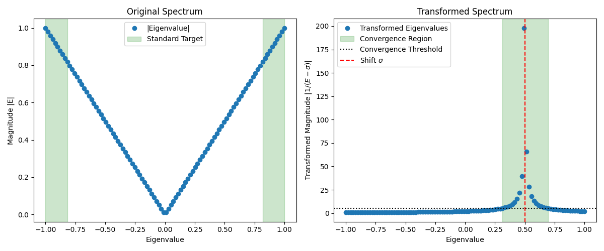
The most common technique is the shift-and-invert method, which transforms the problem $(H - \sigma I)x = \lambda x$ into finding the largest eigenvalues of $(H - \sigma I)^{-1}$. This maps eigenvalues near the shift $\sigma$ to large values, making them accessible to iterative solvers.

We can visualize this effect in the figure below. The left panel displays the original spectrum, where standard solvers naturally target the largest magnitude eigenvalues at the edges (shaded in green). The target eigenvalues near the shift $\sigma$ (red dashed line) are in the interior and difficult to reach. The right panel shows the transformed spectrum $|1/(E - \sigma)|$. Here, the eigenvalues closest to $\sigma$ have been mapped to the largest values (shaded in green), making them the easiest for the solver to find.

However, this requires solving linear systems, which usually involves matrix factorizations (like LU or Cholesky). For large many-body systems, the Hamiltonian $H$ grows exponentially with system size. Explicitly storing or factoring $H$ becomes computationally prohibitive. In these cases, we need "matrix-free" methods that only require matrix-vector products.

Polynomial filtering

This is where polynomial filtering comes in. Instead of inverting the matrix, we construct a polynomial operator $P(H)$ that acts as a filter, amplifying the part of the spectrum we are interested in while suppressing the rest. The ideal filter would be a Dirac delta function $\delta(H - E_{target})$ or a box function, but these are not directly realizable.

We can approximate these filters using a Chebyshev polynomial expansion. Chebyshev polynomials are preferred because they provide the optimal uniform approximation (minimax property) for functions on a finite interval. This allows us to construct a high-order polynomial filter that can be applied to a vector using only repeated matrix-vector multiplications, avoiding expensive factorizations entirely.

We can visualize the action of the Chebyshev filter in the figure below. The left panel shows the original spectrum, where standard solvers naturally target the extremal eigenvalues (shaded in green). The right panel displays the filtered spectrum $|P(E)|$ using a Chebyshev polynomial approximation of a delta function centered at the target $\sigma$ (red dashed line). The filter amplifies the eigenvalues near $\sigma$, mapping them to the largest magnitude values (shaded in green), which are then easily targeted by the eigensolver.

info

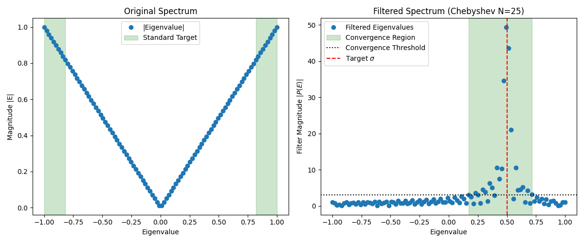
Finite Chebyshev series approximations show oscillations as seen in the figure above. These can be reduced by schemes like Jackson damping. This tutorial does not cover this in detail, but interested readers can refer to the literature on Chebyshev filtering and spectral methods for more information (see Schofield et al.).

Mid-spectrum calculation

We now have all the ingredients to compute mid-spectrum eigenvalues using Chebyshev filters. In the following example, we will demonstrate this process by targeting the central part of the spectrum of a quantum spin chain.

Model Hamiltonian

We will use a 1D spin chain with next-nearest-neighbor interactions. The Hamiltonian is given by: $H = \sum_i \left( X_i + h Z_i + J Z_i Z_{i+1} + \frac{J}{4} Z_i Z_{i+2} \right)$ We choose $L=10$ sites, $J=0.3$, and $h=2J$. Since the system is small, we can compute the exact spectrum for comparison.

    var L = 10
    var J = 0.3
    var h = 2 * J

    var H = operator_sum(as_real);
    for (i : [0..L]) {
        H += X(i)
        H += h * Z(i)
        if (i < L - 1) {
            H += J * ZZ(i, i + 1)
        }
        if (i < L - 2) {
            H += (J / 4) * ZZ(i, i + 2)
        }
    }

    var Hmat = matrix(H, as_real);
    var exact_results = eigensolver(Hmat, ["is_hermitian" : true])

Spectral bounds

To use Chebyshev polynomials, we must first map the spectrum of $H$ to the domain $[-1, 1]$ where the polynomials are defined. This requires estimating the spectral bounds (minimum and maximum eigenvalues) of $H$. If the actual eigenvalues lie outside the estimated range, the Chebyshev series will grow rapidly outside the interval $[-1, 1]$. Consequently, the eigensolver will likely converge to these outlying eigenpairs instead of the desired target states.

We can estimate these bounds using a few iterations of a standard eigensolver targeting the largest magnitude eigenvalues. We add a small buffer to the computed bounds to ensure all eigenvalues fall strictly within the convergence interval of the Chebyshev series.

    var lbound = 0.0
    var ubound = 0.0
    {
        var results = iterative_eigensolver(H, 2**L, 1, ["is_hermitian" : true, "is_real" : true])
        lbound = results[0].value() // value extracts the eigenvalue from the matrix object
    }
    {
        var results = iterative_eigensolver(H, 2**L, 1, ["is_hermitian" : true, "is_real" : true, "spectrum" : spectrum.largest_real])
        ubound = results[0].value()
    }

    print("| Bound | Exact | Iterative |")
    print("|-------|-------|-----------|")
    print("| min  | ${min(exact_results.eigenvalues())} | ${lbound} |")
    print("| max  | ${max(exact_results.eigenvalues())} | ${ubound} |")

info

Here, we use a low tolerance to obtain nearly exact spectral bounds. For larger systems, one might consider increasing the tolerance to save time, adding a buffer to ensure all eigenvalues fall within the Chebyshev expansion interval. However, since computing a few extremal eigenvalues is typically not a bottleneck for the overall calculation, strict tolerances are usually affordable.

Determining the filter function

We will use a "delta" filter approximated by a Chebyshev series. This filter peaks at a target energy and decays rapidly away from it. The function chebyshev_series_delta generates the coefficients for this expansion. The degree of the polynomial, npoly, determines the sharpness of the filter. A higher degree resolves the target eigenvalues better but increases the computational cost (requiring more matrix-vector products). The dimension of the Krylov subspace, nsub, for the eigensolver must be large enough to accommodate the number of eigenvalues, nev, we expect to find under the filter's peak. A good rule of thumb is to use a subspace size of 2-3 times the number of desired eigenvalues.

    var npoly = 25
    var nev = 50
    var nsub = 2 * nev
    var buffer = (ubound - lbound) * 0.01
    var cheb_series = chebyshev_series_delta(npoly, interval(lbound - buffer, ubound + buffer))

info

Although a higher polynomial degree increases the cost of applying the filter, it results in a sharper spectral peak. This improved resolution often accelerates the eigensolver's convergence by effectively isolating the target eigenvalues, which can lead to a reduction in overall computation time.

In this example, we choose a polynomial degree of npoly = 25, which is sufficient to resolve the nev = 50 target eigenpairs for this system. We set the Krylov subspace dimension nsub to 2 times the number of desired eigenvalues to ensure robust convergence. While these parameters work well here, the optimal choice depends on the specific problem, the density of states near the target energy, and available computational resources. Users are encouraged to experiment with these parameters for their particular applications.

To understand how to choose these parameters, consider how iterative eigensolvers behave. They are generally effective at converging on clusters of eigenvalues – whether a single isolated eigenvalue or a group of closely spaced ones. However, if the Krylov subspace is too small to accommodate an entire cluster of tightly packed eigenvalues, convergence will suffer. For example, if you seek 5 eigenvalues but they are part of a cluster of 10, the solver may struggle as the states "compete" for space in the subspace.

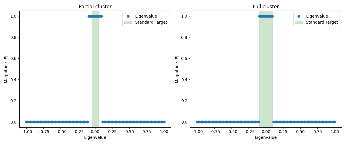
Consider the following figure illustrating two scenarios:

note

Graphing tools will soon be available in Aleph. Stay tuned to know how to create such plots directly within Aleph.

In both cases, we have a filter that isolates eigenvalues in the interval $[-0.1, 0.1]$.

• Left: We target a subset of the cluster (interval $[-0.05, 0.05]$) with a small Krylov subspace. Convergence is difficult because the subspace barely accommodates the target pairs, and the solver struggles to separate them from the rest of the cluster.
• Right: We target the entire cluster (interval $[-0.1, 0.1]$) and allocate a larger Krylov subspace. Although each iteration is more expensive due to the larger subspace, convergence is typically much faster and more robust because the entire cluster fits comfortably.

The first scenario effectively requires a "filter on top of a filter" to isolate the specific subset, which is numerically difficult. It is often better to broaden the target range (or increase the subspace size) to capture the full cluster, rather than trying to "slice" through it.

Let's apply this to our example. The following plot shows the density of states of our Hamiltonian.

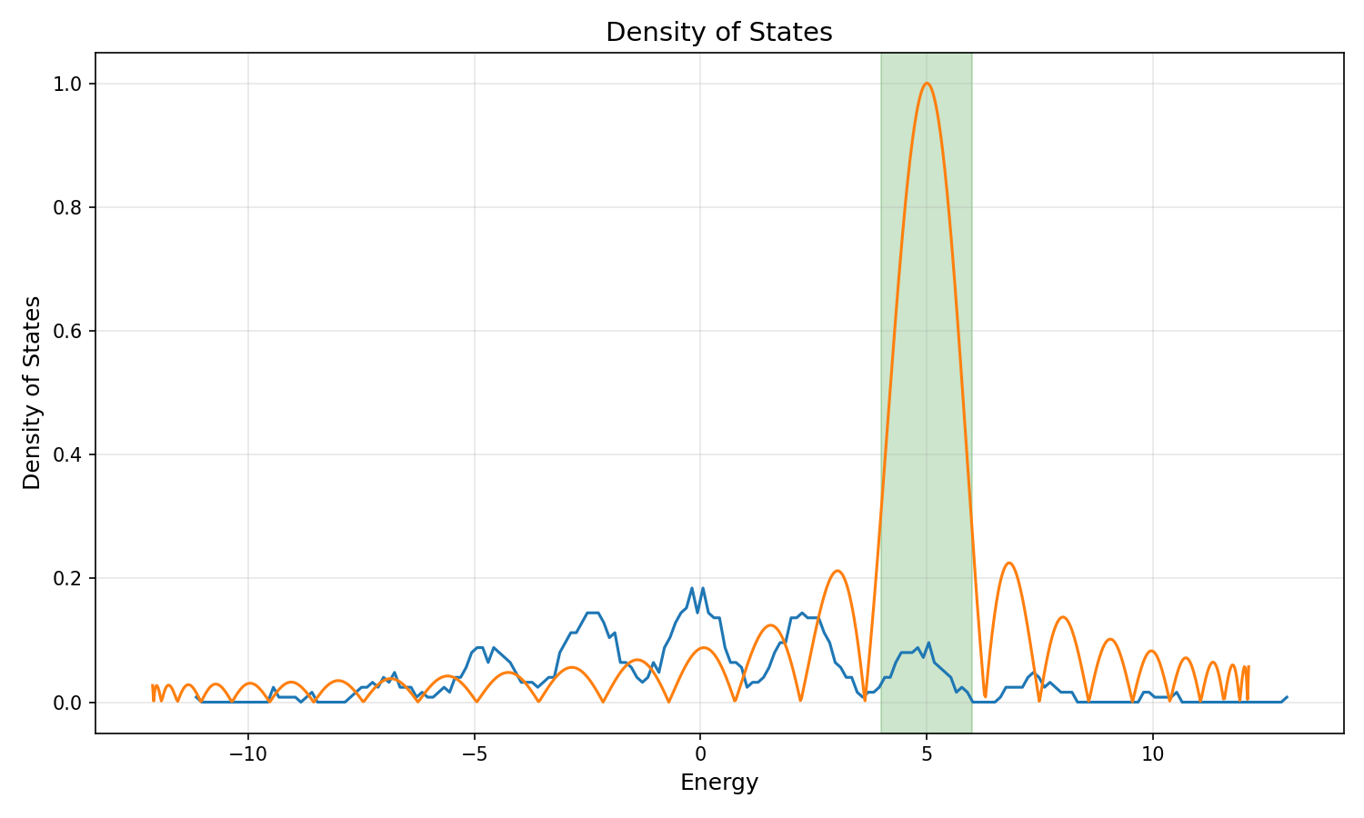
The density of states exhibits peaks and dips. When selecting the target energy, it is important to consider these features. We will focus on the peak between energies 4 and 6. We use a Chebyshev filter of degree 25 centered around 5. This filter peaks at 5 and decays away from it, effectively isolating the eigenvalues in that region. There are roughly 100 eigenvalues in the interval $[4, 6]$. By seeking nev = 50 eigenvalues with a sufficiently large subspace (or by adjusting our filter to be sharper), we ensure that the solver can isolate the states we are interested in.

info

For many-body Hamiltonians, the spectral width typically scales linearly with system size, whereas the Hilbert space dimension grows exponentially. Consequently, the density of states becomes increasingly concentrated near the center of the spectrum. When targeting mid-spectrum eigenvalues in larger systems, this necessitates adjusting both the polynomial degree and the Krylov subspace size. Specifically, a higher polynomial degree is required to construct a sufficiently narrow filter, and a larger Krylov subspace is needed to accommodate the growing number of eigenvalues within the target window. The table below illustrates how the required polynomial degree (N series) scales with system size (N sites) when targeting 1000 mid-spectrum eigenvalues for a similar Hamiltonian:

N sites	N eigenvalues	N series
14	1000	28
16	1000	106
18	1000	400
20	1000	1518
22	1000	5790
24	1000	22150

Here, the Krylov subspace size was set to three times the number of desired eigenvalues in all cases. Since the Krylov subspace size is limited by the computer's available memory, as the system size increases, the polynomial degree required to effectively isolate the target eigenvalues grows significantly due to the increasing density of states in the mid-spectrum region.

Diagonalize the filter

Finally, we construct the filter operator using operator_chebyshev_series. This function returns an operator that applies the polynomial filter $P(H)$ to a vector. We then use a standard iterative eigensolver on this new operator.

info

One might ask why we do not use a generic polynomial operator that accepts arbitrary polynomial coefficients, rather than specifically a Chebyshev series. The reason is numerical stability. Evaluating high-order polynomials directly is prone to numerical instability, especially near the edges of the interval $[-1, 1]$. Chebyshev polynomials can be evaluated with the Clenshaw algorithm, providing a numerically stable basis for polynomial approximation, allowing us to evaluate the filter operator accurately even at high degrees. The operator_chebyshev_series function creates an operator that implements a version of the Clenshaw algorithm that computes matrix-vector products.

The eigensolver will find the eigenvectors of $P(H)$, which are identical to the eigenvectors of $H$. However, the eigenvalues will be the filtered values $P(E)$. To recover the original energies $E$, we compute the expectation value $\langle \psi | H | \psi \rangle$ for each eigenvector.

    var cheb_operator = operator_chebyshev_series(H, cheb_series)
    var results = iterative_eigensolver(cheb_operator, 2**L, nev, ["is_hermitian" : true, "is_real" : true, "spectrum" : spectrum.largest_real, "krylov_dimension" : nsub])

We verify the results by checking that the computed eigenvectors are indeed eigenvectors of the original Hamiltonian and that the recovered eigenvalues match the exact ones.

    var evecs = results[1];

    // Check that evecs are eigenvectors of the filtered operator
    var filtered_evals = results[0];
    var conv = is_approx(cheb_operator * evecs, evecs * filtered_evals.as_diagonal(), 1e-8)
    if (!conv) {
        print("Eigenvectors are not eigenvectors of the filtered operator")
    }

    // Recover the original eigenvalues (energies)
    var energies = (evecs.adjointed() * (H * evecs)).diagonal();
    var exact_evals = array(exact_results.eigenvalues())

    // Check that all recovered energies match an exact eigenvalue
    for (E : energies)
    {
        if (min(abs(E - exact_evals)) > 1e-8) {
            print("Eigenvalue ${E} not found in exact spectrum")
        }
    }

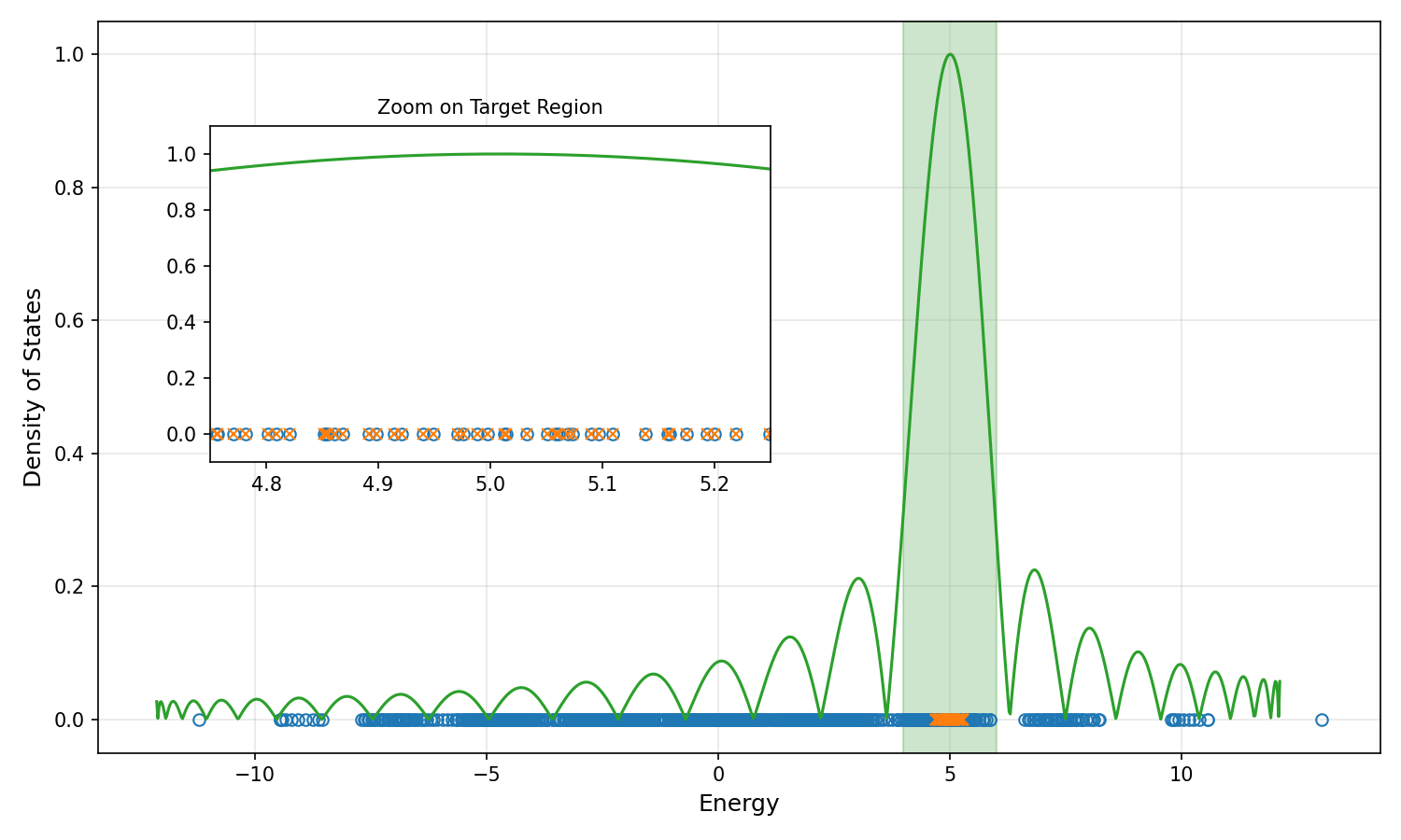
Let's visualize the results. The following plot shows the original eigenvalues (crosses) and the exact eigenvalues (circles) in the target region, along with the Chebyshev filter used. The inset zooms in on the target region to show how well the filter isolates the desired eigenvalues. It does not show the full target region for clarity, as eigenvalues are densely packed there.

Summary

In this tutorial, we demonstrated how to compute mid-spectrum eigenvalues of a many-body Hamiltonian using Chebyshev polynomial filtering. This matrix-free approach avoids the need for expensive matrix factorizations, making it suitable for large systems where traditional shift-and-invert methods are impractical. By carefully selecting the polynomial degree and Krylov subspace size, we effectively isolated and computed the desired interior eigenvalues. This technique is a powerful tool for exploring excited state properties in quantum many-body systems.

What's next?

• Parameter exploration: Vary the polynomial degree npoly and the Krylov subspace size nsub. How do these parameters affect the accuracy of the eigenvalues and the convergence speed? Try to reproduce the "cluster" convergence issues discussed earlier by intentionally choosing a small subspace (you may have to increase system size to get enough "clustering", Krylov methods are pretty robust!).
• Entanglement scaling: Compute the entanglement entropy of the mid-spectrum eigenstates using reduced_density_matrix and von_neumann_entropy. Compare the scaling of entropy with system size $L$ for mid-spectrum states versus the ground state. This is a signature of the difference between thermalizing (volume-law) and localized (area-law) phases.
• System size scaling: Try to push the simulation to $L=20$ or $L=22$. Use the table provided in the tutorial to estimate the required polynomial degree. How does the runtime scale?
• Different models: Apply this technique to a different Hamiltonian, such as the Heisenberg model with a random magnetic field (a standard model for Many-Body Localization). How does the density of states changes?